Inland harmful algal blooms (HABs) modeling using internet of things (IoT) system and deep learning

Article information

Environmental Engineering Research. 2023;28(1)

Publication date (electronic) : 2022 January 26

doi : https://doi.org/10.4491/eer.2021.280

Do Hyuck Kwon ¹, Seok Min Hong ¹, Ather Abbas ¹, JongCheol Pyo ², Hyung-Kun Lee ³, Sang-Soo Baek ⁴^,

¹School of Urban and Environmental Engineering, Ulsan National Institute of Science and Technology, Ulsan, 44919, Republic of Korea

²Center for Environmental Data Strategy, Korea Environment Institute, Sejong 30147, Republic of Korea

³ICT Materials and Components Research Laboratory, Electronics and Telecommunications Research Institute (ETRI), Daejeon, Republic of Korea

⁴Department of Environmental Engineering, Yeungnam University, 280 Daehak-Ro, Gyeongsan-Si, Gyeongbuk 38541, Republic of Korea

^†Corresponding author: E-mail: khcho@unist.ac.kr; kbcqr@naver.com, Tel: +82-52-217-2829; +82-52-217-2886, Fax: +82-52-217-2819; +82-52-217-2819

Received 2021 June 13; Revised 2021 October 19; Accepted 2022 January 20.

Abstract

Harmful algal blooms (HABs) have been frequently occurred with releasing toxic substances, which typically lead to water quality degradation and health problems for humans and aquatic animals. Hence, accurate quantitative analysis and prediction of HABs should be implemented to detect, monitor, and manage severe algal blooms. However, the traditional monitoring required sufficient expense and labor while numerical models were restricted in terms of their ability to simulate the algae dynamic. To address the challenging issue, this study evaluates the applicability of deep learning to simulate chlorophyll-a (Chl-a) and phycocyanin (PC) with the internet of things (IoT) system. Our research adopted LSTM models for simulating Chl-a and PC. Among LSTM models, the attention LSTM model achieved superior performance by showing 0.84 and 2.35 (μg/L) of the correlation coefficient and root mean square error. Among preprocessing methods, the z-score method was selected as the optimal method to improve model performance. The attention mechanism highlighted the input data from July to October, indicating that this period was the most influential period to model output. Therefore, this study demonstrated that deep learning with IoT system has the potential to detect and quantify cyanobacteria, which can improve the eutrophication management schemes for freshwater reservoirs.

Keywords: Attention mechanism; Deep learning; Harmful algal blooms (HABs); Internet of things (IoT); Water quality

1. Introduction

The outbreak of harmful algal blooms (HABs) adversely affected water quality in rivers and lakes [1]. HABs have been frequently reported at global scale according to rapid urbanization and global climate change [2, 3]. The algae can release toxic substances, which typically lead to water quality degradation and health problems for humans and aquatic animals [4]. Since the construction of a multi-functional dam and weir in major rivers of South Korea, the country has experienced cyanobacteria outbreaks, which release microcystin, a toxic substance that negatively affects the human body [5]. In particular, Daechung reservoir in South Korea has annually endured the outbreak of HABs due to the inflowing massive nutrient and warm water [6]. Hence, an accurate quantitative and qualitative analysis of HABs via monitoring should be implemented to detect, monitor, and regulate severe algal blooms [7–9].

South Korea equips the algal alert system to monitor water quality for securing public health and drinking water. This monitoring system has weekly measured water quality related to HABs and notifies the government agency of the observation [10]. However, the weekly monitoring cannot identify the instant change of HABs because the dynamic of HABs has high variation and uncertainty [11]. In addition, persistent HABs monitoring is time consuming, costly, and labor intensive [12]. Recently, the internet of things (IoT) platform including detection sensors and wireless network has been proposed as a promising monitoring technique, since it is capable of receiving the real-time data of water quality [13, 14]. Hu et al. [15] acquired water quality data through the real-time monitoring using the detection sensors and the mobile online servers. They have collected real-time data such as water temperature, dissolved oxygen, salinity, and pH level. Although the real-time monitoring system can be useful to identify the deterioration of water quality, few studies have applied this technique to HABs monitoring.

Given the limited resources, understanding HABs via simulation could be useful to control the outbreak of algae [16]. The simulation of water quality through modeling regards important to determine the policy decisions for effective water resources management. Previous studies have developed numerical-based water quality models to understand the dynamics of algae, including the Environmental Fluid Dynamics Code (EFDC), Soil Water Assessment Tool (SWAT), and CE-QUAL-W2 [17–19]. However, these models were restricted in terms of their ability to simulate algal dynamics [5, 20, 21]. Additionally, these models have a challenging issue regarding the complexity of HAB dynamics depending on multiple physical, chemical, and biological system effects [10, 22]. To address this challenge, the data-driven model has been introduced as an alternative approach to predict water quality and HABs by learning non-linear mathematical relations between input and output data [23]. Specifically, long Short-Term Memory (LSTM) has a considerable advantage in the time-series data [24]. Baek et al. [25] simulated the water level, total nitrate (TN), total phosphorus (TP), and total organic carbon (TOC) using LSTM. Zhang et al. [26] utilized the LSTM model to predict the water level in the urban drainage system. However, these models are limited to explain the correlation between input and output variables, and the observation [27, 28]. Data preprocessing also has an important role in machine learning and deep learning algorithms, and proper data preprocessing is compulsory for achieving better model performance [29]. Shen et al. [30] demonstrated that it is necessary to use the preprocessing method for managing big data prior to the application of data-driven models.

Hence, we aim to evaluate the applicability of deep learning to simulate chlorophyll-a (Chl-a) and phycocyanin (PC) concentrations with real-time monitoring in Daechung reservoir, South Korea. Chl-a and PC are the proxy indicator of the algal biomass, Chl-a is an indicator of phytoplankton biomass and PC is an accessory pigment of cyanobacteria [31, 32]. Our research adopted state-of-the-art data-driven models, attention LSTM. the attention mechanism is the overcoming approach with explainability by analyzing the features of attention weight [33]. In this regard, the main objectives of our research were to: (1) conduct HABs monitoring via IoT system, (2) simulate Chl-a and PC concentrations using LSTM models, (3) evaluate the model performance depending on the data preprocessing method, and (4) interpret the model result through attention weights of the model.

2. Material and Methods

2.1. Study Area and Data Acquisition

Daechung reservoir is located in upstream of Geum River, South Korea (N 36.35–36.52, E 127.48–127.60) (Fig. 1). This reservoir has supplied water to nearby cities (e.g. Daejeon and Chungju) for agricultural, domestic, and industrial use [34]. The water surface area and storage capacity are 72.8 km² and 1,490 × 10⁶ m³, respectively [35]. This site has the frequent occurrences of HAB from summer to late autumn [36]. The HABs by cyanobacteria have been annually reported during this season as regular events [37]. We measured Chl-a, PC, and seven water quality variables at two stations: Hoenam and Chusori. Hoenam is a transition zone that flows into the reservoir in the mainstream of the Geum River [38, 39]. Chusori has inflow from excessive anthropogenic sources including the sewage treatment water and fertilizers [40]. The monitoring was conducted from January to December in 2020. TN and TP were obtained by Ministry of Environment [41]. Meteorological data were acquired from near weather stations (e.g., Secheon (N 36.35–36.52, E 127.48–127.60) and Cheongnamdae (N 36.35–36.52, E 127.48–127.60)) [42]. Daily inflow and outflow of the reservoir were measured by the Water Resources Management Information System [43].

Fig. 1

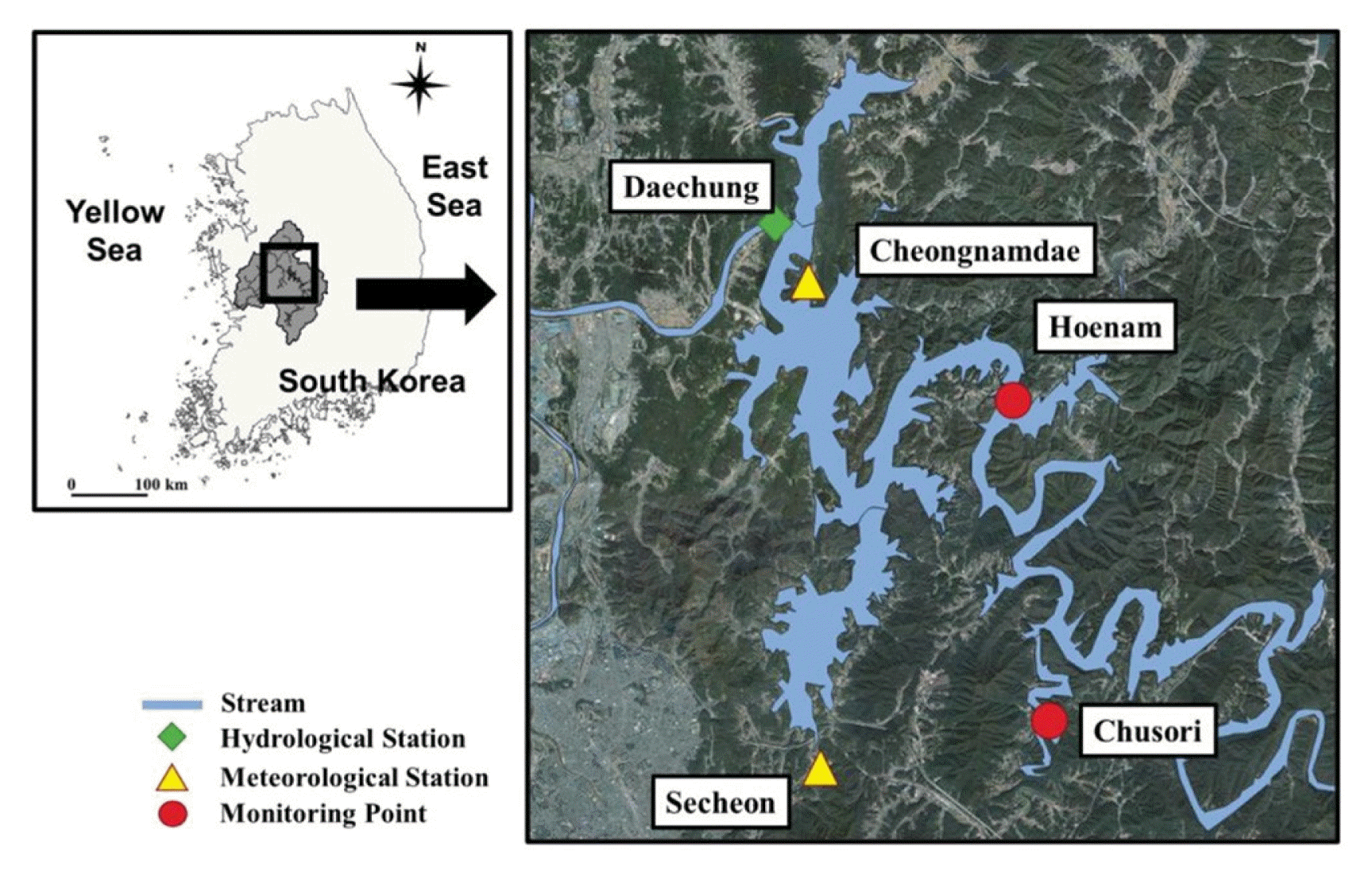
Study area: Daechung reservoir with hydrological stations, meteorological stations, and monitoring points. Green diamond, yellow square, and red circle indicate the hydrological station, the meteorological station, and the monitoring point, respectively.

2.2. Internet of Things (IoT) Monitoring for Harmful Algal Blooms (HABs)

Fig. 2 describes the pontoon monitoring system consisting of a multi-parameter water quality instrument (EXO-2) and a remote terminal unit (RTU). EXO-2 (YSI Inc., Yellow Springs, Ohio, USA) can measure seven water quality variables: water temperature (WT) (°C), pH, electrical conductivity (EC) (mS/cm), dissolved oxygen (DO) (%), turbidity (Turb) (FNU), Chl-a (μg/L) and PC (μg/L) (Table S1). The water quality data are collected with RTU (Deongmoon ENT Co., ECO::WATCH RTU V3, Seoul, Korea) on the pontoon and transmitted to a data server through NB-IoT model [44, 45]. The RTU manages data collection schedule of EXO-2 and power-supply level of pontoon system. The NB-IoT module (SERCOM Co., TPB22-3) is used for low-power and long-distance wireless data communication. Real-time water quality monitoring using pontoon was conducted on the water surface. The water quality sensor of the pontoon was installed from 0.5 to 1.8 m.

Fig. 2

Pontoon monitoring system in Daechung Reservoir. (a) pontoon monitoring system for measuring water quality variables; (b) pontoon monitoring system in study site; (c) YSI-EXO-2 multi-parameter water quality instrument.

2.3. Chlorophyll-a and Phycocyanin Simulation Using Deep Learning

The deep learning for simulating Chl-a and PC consisted of four steps: (1) preparation of input data (Fig. 3(a)), (2) data preprocessing (Fig. 3(b)), (3) hyperparameters optimization (Fig. 3(c)), and (4) simulation of Chl-a and PC using deep learning (Fig. 3(d)). This study used seven water quality, two hydrological, and two meteorological as input data for simulating Chl-a and PC (Table S1). These hydrological and environmental data have verified the factors to influence algal growth [46]. Prior to application of deep learning, the input data applied three data preprocessing: min-max, z-score, and robust scaling methods. The min-max method rescales the data set with the range of zero to one using minimum and maximum values [47]. The z-score uses the mean and the standard deviation, thereby the mean value calculates zero. The robust scaling removes the outlier in the dataset and calculates with interquartile range. In addition, this study optimized five hyperparameters using the bayesian optimization algorithm (Table S2). The hyperparameters can control the learning process and backpropagation [48, 49]. Finally, we simulated Chl-a and PC concentrations using three deep learning models: attention LSTM, one-layer LSTM, and two-layer LSTM. In our study, the dataset was randomly assigned to training and validation set from the observation. Previous studies have also used random sampling to divide the training and validation [50, 51]. Therefore, our dataset was divided into 70% of training and 30% of validation by random sampling. Our models have been trained using the adam optimizer to update the model weight and parameters to reduce loss value [52]. We used version 2.10 of Tensorflow API in the Python programming language to build up the deep neural network models [53]. Our model training was performed using an Intel® Core i9-10900F 2.80 GHz processor, the DDR4 64 Gigabytes of random-access memory, and NVIDIA GeForce RTX 3070 graphic card.

Fig. 3

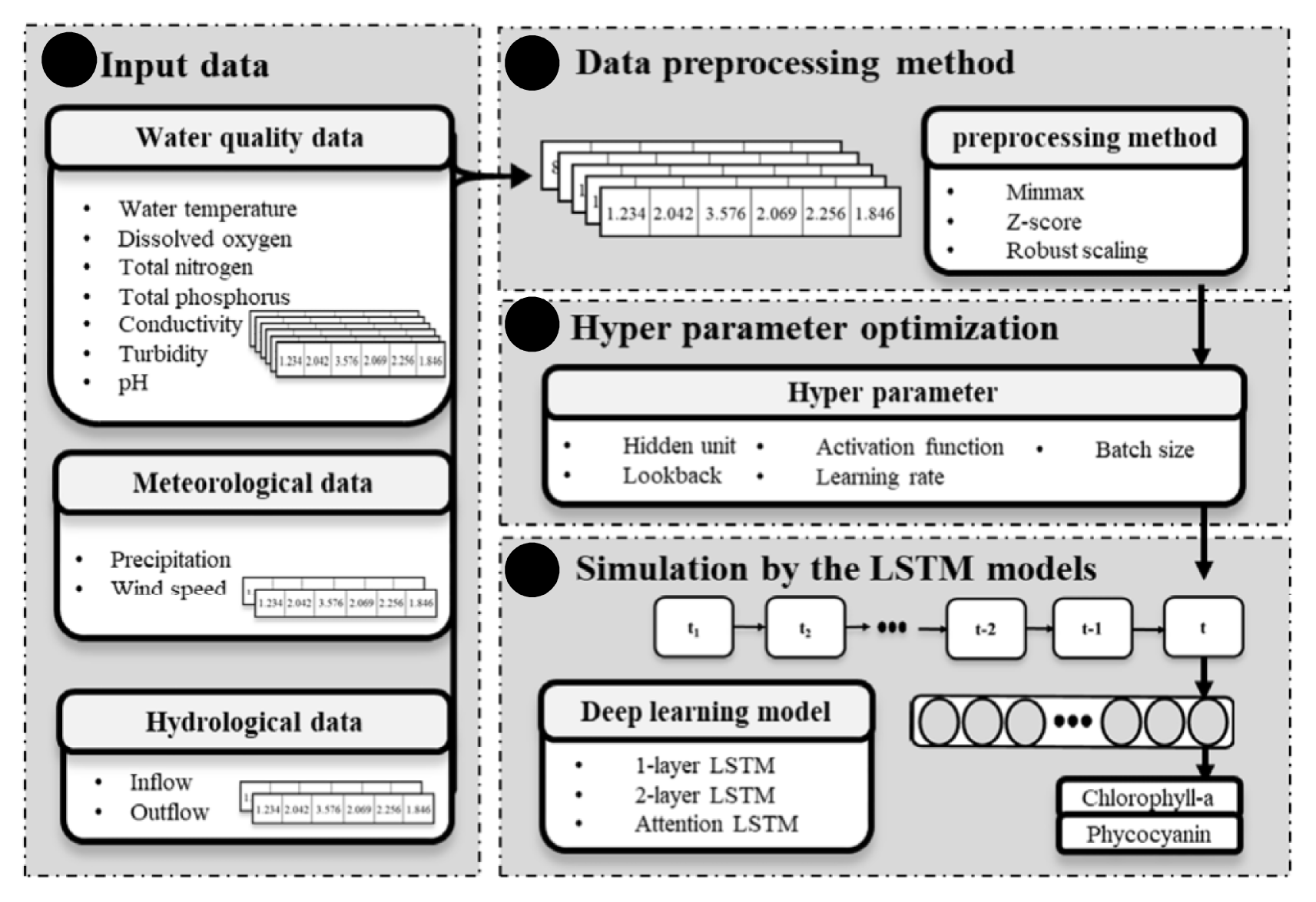
Schematic diagram for simulating Chl-a and PC concentration.

2.3.1. Data preprocessing

The environmental variables have high variation with biased or skewed distribution, resulting in the biased model training [54]. These problems cause the presence of outliers, missing values, and non-normal distribution, which has led to a deviation between the input dataset [55, 56]. To solve this problem, this study applied three preprocessing methods: the min-max, z-score, and robust scaling methods. Previous studies demonstrated that the application of data preprocessing can guarantee the data quality before feeding into the deep learning model to minimize data variability [57]. The min-max linearly transforms original data using minimum and maximum values [58]. The min-max function is expressed as follows:

(1) Y(x)=xi-min(x)max(x)-min(x)

where Y(x) is the normalized value. x_i is the data. The min(x) and max(x) are minimum and maximum of data. The technique provides the normalized value from zero to one.

The z-score transforms the data using the mean and the standard deviation [47]. The z-score is expressed as follows [59]:

(2) Y(x)=xi-mean(x)standard deviation(x)

where the mean(x) is the mean of the data and the standard deviation( x) is the standard deviation of data [47].

The robust scaling could consider the presence of outlier using the interquartile range (IQR) that is the difference between the 1^st quartile and 3^rd quartile, thereby minimizing the impact of outliers [60]. This equation is expressed as:

(3) Y(x)=xi-Q1(x)Q3(x)-Q1(x)

where Q₁ is the 1^st quartile and Q₃ is the 3^rd quartile.

2.3.2. Attention LSTM

Attention LSTM is the version of coupled LSTM and attention mechanism (Fig. 4 (a)). In the attention LSTM, the previous information are recurrent to deal with the sequence data by the LSTM layer (Fig. 4(b)). Additionally, this model was combined with the attention mechanism that is known to be used to enhance the model performance and interpretability (Fig. 4(c)) [61]. The attention mechanism decides the significant part of input data during the model training. In addition, this mechanism can explain the model result by generating the attention score map that can visualize the importance of input data [62]. Vaswani et al. [63] demonstrated that attention-based models had faster training time than existing recurrent and convolutional neural networks. The following equations are used to calculate the attention mechanism:

Fig. 4

Descriptions of LSTM and attention LSTM; (a) attention LSTM, (b) LSTM mechanism, and (c) attention mechanism.

(4) etk=vet·tanh (We[ht-1;st-1]+Ue·yk)

(5) atk=exp (etk)Σi=1nexp (eti)

(6) Ct=Σi=1matk hi

where the e_t and t are alignment score, and the sequence length of input, respectively. atk is a softmax function that turns an array of alignment scores to sum with one [64]. The parameters v_e, W_e, and U_e are the weight matrices determined by the training process and the y^k indicates the number of input data. The and C_t are h_i context vector and hidden state, respectively.

2.3.3. Long short-term memory (LSTM)

LSTM is developed based on recurrent neural network (RNN) [65]. The RNN is designed to deal with sequence data by interrelating between the previous state and the current state [66]. The RNN contains a recurrent loop, regulating information to be stored within the network. RNNs are weak to learn the long sequence due to the vanishing gradient problem in the deep neural network which means that previous data is not reflected in the current state [67]. The LSTM is proposed for resolving the vanishing gradient problem by applying gates in RNN cells. The LSTM architecture is composed of three gates namely forget, update, and output gate to regulate the interaction of the previous information. The LSTM can be calculated by the following equations:

(7) ft=σ (Wi[ht-1,xt]+bi)

(8) it=σ (Wi·[ht-1,xt]+bi)

(9) c¯t=tanh (Wc·[ht-1,xt]+bc)

(10) ct=ft×ct-1+it×c¯t

(11) ot=σ (Wo·[ht-1,xt]+bo)

(12) ht=ot×tanh (ct)

where f_t is the forget gate, which determines what information should be forgotten or not. The previous hidden state and information from current input, x, pass through the sigmoid function, σ, which ranges from zero to one. The input gate, i_t, is the process of deciding whether to store current information using the sigmoid function. Tangent hyperbolic function, tanh, helps to regulate the network in the new memory cell, c̄_t. Then, the current cell state, c_t, can be updated with the forget and input gate to contain information of current and previous state. o_t denotes the activation vectors of the output gate to adjust the output activation of the cell. The W and b indicate weight and bias that can be calculated during the model training. The parameters h and c mean the hidden states and cell states [68].

2.3.4. Hyper-optimization (HPO)

The hyperparameters have strongly influenced the performance of data-driven models [48]. We obtained the optimal hyperparameter set using the bayesian optimization method [49, 69]. The bayesian optimization algorithm is derivative-free optimization to find the optimal hyperparameters with the gaussian process [70]. The hyperparameter is tuned to minimize the loss value within the configured range, thereby selecting the parameter to improve the performance of models [71]. In our study, Table S2 describes the hyperparameter range for HPO. The hyperparameters were automatically searched for the optimal value during bayesian optimization process. The mean square error (MSE) was adopted for calculating the loss between simulation and observation [72]. Also, we applied the dropout of 0.3 to prevent the overfitting problem [73]. Libraries of scikit-optimize and Hyperopt were used for HPO [74].

2.4. Model Evaluation

The model performance was evaluated using the correlation coefficient (R) and root mean square error (RMSE). The R and RMSE can represent the indices for the relationship and error between the observation and the simulation [75]. These indices are obtained using the following equations:

(13) R=1-Σt=1n(ot-pt)Σt=1n(ot-p¯t),-1.0≤r≤1.0

(14) RMSE=∣Σi=1∣n(oi-pi)2n

where p_t is the simulated data, o_t is the observed data, p̄_t is the mean of the simulated data, and n is the number of data. This study adopted the Taylor diagram to visualize the model performance, which can express the geometric relationship [76].

3. Result and Discussion

3.1. Real-time Monitoring for Algal Bloom

The boxplots of Chl-a and PC concentration are presented in Fig. S1. The mean concentrations of Chl-a and PC in Hoenam are 4.47 μg/L and 0.07 μg/L, respectively, and those in Chusori were 9.51 μg/L and 1.32 μg/L, respectively. The Chl-a and PC concentrations in Chusori increased from late summer to autumn, yielding 97.56 μg/L and 31.37 μg/L of peak concentrations, respectively. These concentration levels can be regarded as the ‘very bad’ level according to ambient water quality standard in South Korea [77]. This was caused by high temperature and excessive nutrient loading by heavy rainfall [78, 79]. The water temperature in this study ranged from 23°C to 31°C when HABs occurred. This range of water temperature can strongly affect the growth rate of algae, the vertical mixture of the freshwater, and the reduction of viscosity [80]. Pawlita-Posmyk et al. [81] referred that the warm water temperature between 15°C to 26°C can promote algal growth. The peak nutrient concentrations were observed in this bloom period; Hoenam showed TN and TP of 2.59 mg/L and 0.08 mg/L, respectively, and Chusori showed that of 4.06 mg/L and 0.20 mg/L. It implies that our study sites received excessive nutrients from the watershed, resulting in the outbreak of cyanobacteria bloom [82]. Paerl et al. [83] demonstrated that the growth of cyanobacteria might have positive relationship with nutrients because this species can use nitrogen and phosphorus to increase biomass.

3.2. Effect of Data Preprocessing

We compared the model performance using the Taylor diagram that can visualize the statistical summary between the observation and simulation (Fig. 5) [84]. Attention LSTM with the z-score showed the highest model performance by having the highest value of R and the lowest value of RMSE; the average values of R and RMSE were 0.84 and 2.35 (μg/L), respectively. It implies that the attention LSTM and z-score were suitable to simulate Chl-a and PC. Ding et al. [85] and Luong, Pham and Christopher [61] presented that the attention mechanism improved performance compared to the other models because this mechanism can be useful to capture the feature of input data. Zhang et al. [86] demonstrated that the z-score can stabilize the model training by reliving the negative effect of the outlier. In the contrast, the 2-layer LSTM and the min-max scaler were improper to simulate HABs, by showing the lowest performance. Especially, the model performance was decreased as increasing the number of layers. It indicates that the complex model might deteriorate the model accuracy than the simple model (i.e., 1-layer LSTM). Cho et al. [87] also showed that the model complexity negatively influenced the model inference, which imposed excessive computation power to identify the important features in data and parameters. Although min-max scaler was popular among preprocessing methods, this method had limited to reduce the effect of outlier and the variation of data [58]. The model performance varied depending on the type of structure and preprocessing. It reveals that the selection of structure and preprocessing method were essential steps for effective model training and application. Chen et al. [88] suggested that the inappropriate selection of them might cause the vanishing gradient, thereby producing worse simulation.

Fig. 5

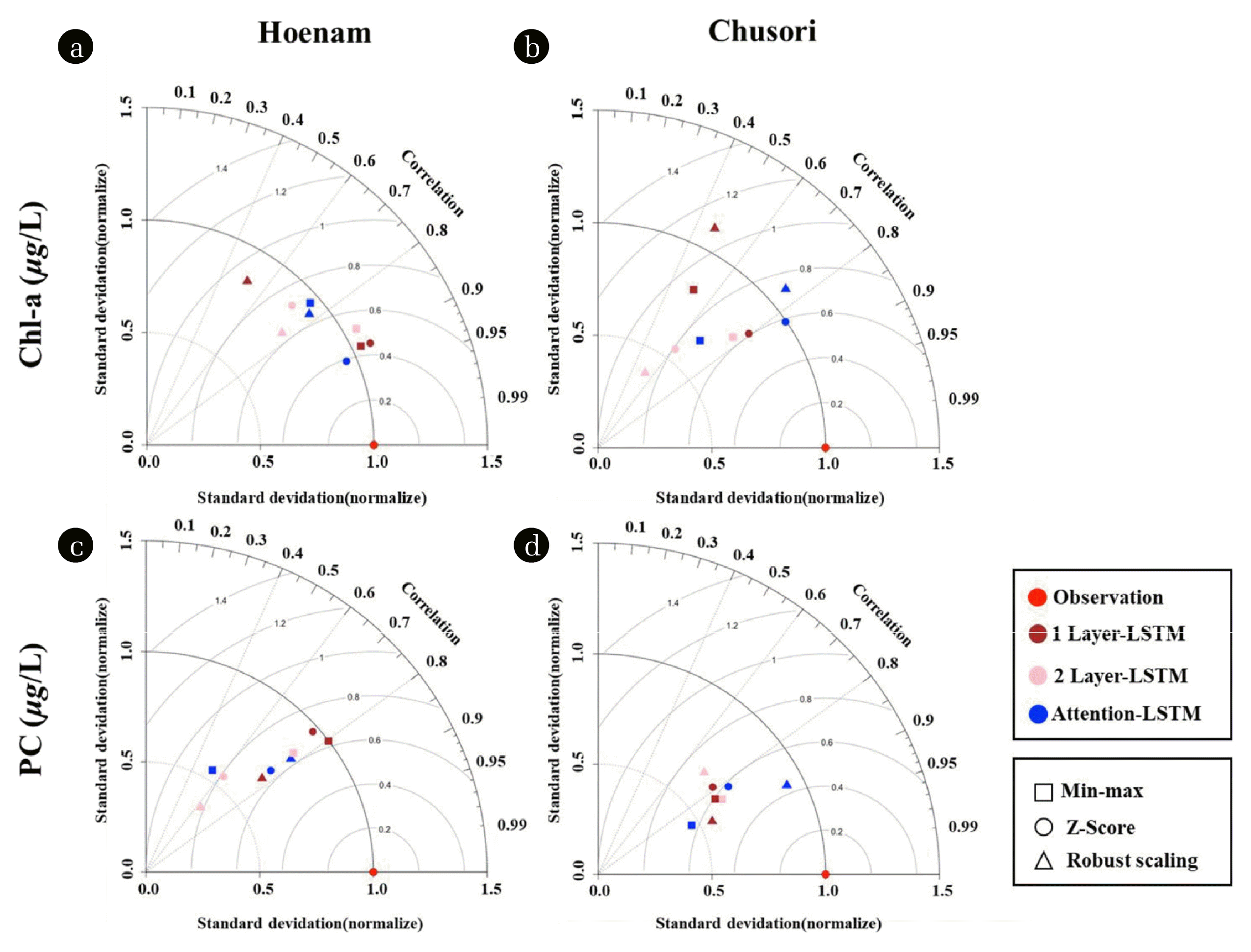
Taylor plots of the LSTM models including correlation coefficient, normalized standard deviation, and centered pattern RMSE. Red, brown, pink, and blue color indicate observation, 1-layer LSTM, 2-layer LSTM, and attention LSTM, respectively, while square, circle, and triangle shapes indicate min-max, z-score, and robust scaling method, respectively.

3.3. Hyper-parameter Optimization

Fig. S2 and S3 show the optimization process using the attention LSTM model with z-score scaling. The learning rate is the most sensitive hyperparameter in that the changed slope is the steepest compared to other parameters. During optimization, the learning rate was converged from the large value to the small value, implying that our model preferred the small step size when adjusting the weight and bias. Jang et al. [89] and Yun et al. [90] also recommended the smaller learning rate to simulate the water quality. In addition, the lookback also was the influential factor to the model result. The lookback can define the value how many previous timesteps to simulate the output value [64]. In the contrast, the model performance was weakly influenced by the type of activation functions. Table S3 describes the optimized hyperparameter value from the optimization process. The optimal batch sizes for Hoenam and Chusori were eight. Previous studies showed that eight of batch size was enough to model training without the vanishing gradient and overfitting problems for the environmental simulation [91]. Our lookback optimal sizes were eight and seven for Hoenam and Chusori, indicating that the HAB simulation required the temporal information from the previous eight and seven days to the current simulation time, respectively.

3.4. Chlorophyll a and Phycocyanin simulation

Fig. 6 and 7 present the time series and scatter plot of Chl-a and PC using attention LSTM with z-score scaling. The simulated Chl-a and PC concentrations were similar to the observation in both sites. On the Hoenam, the R and RMSE showed 0.92 and 1.63 (μg/L) of Chl-a, and 0.77 and 1.66 (μg/L) of PC, respectively. On the Chusori, the R and RMSE showed 0.82 and 3.61 (μg/L) of Chl-a, and 0.83 and 2.48 (μg/L) of PC, respectively. These results implied the acceptable performance and good agreement with the observed Chl-a and PC. In particular, the Chl-a and PC simulation in spring and winter exhibited improved model accuracy compared to the summer season. This is because various external sources (e.g., heavy rainfall, nutrient loading, and warm water) existed that the algae life cycle in the summer season [80]. Park et al. [92] demonstrated that the algae life cycle was significantly influenced by nutrients and discharge from the watershed. The simulated Chl-a concentration showed higher variation than PC concentration from July to October. This is because the concentrations of Chl-a were influenced by the dynamic of diatoms, green algae, and cyanobacteria while PC was an indicator for cyanobacteria that had rapid growth in summer [93]. The Chl-a and PC concentrations in Hoenam had relatively lower concentrations compared to Chusori because Hoenam presented had deep water above 25 m compared to Chusori station, resulting in the shorter retention time [37]. Cha et al. [94] reported that a short retention time might restrict algal growth by accelerating the dispersion and advection of HABs.

Fig. 6

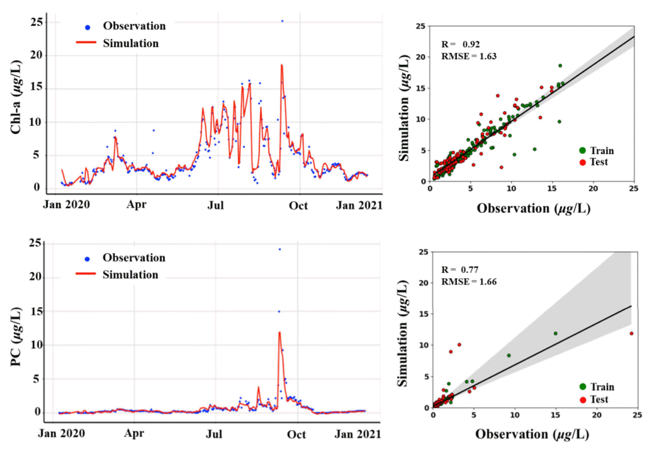
Comparison of simulated Chl-a and PC concentrations in Hoenam with observation.

Fig. 7

Comparison of simulated Chl-a and PC concentrations in Chusori with observation.

3.5. Model Interpretability with Attentions

Fig. 8 shows the attention score map to temporally interpret the attention LSTM model. The plots represent the weight of input data to affect the model output [89]. On the attention score map, the color bar indicates the importance of the dataset [64]. The results were highlighted from June to October in Hoenam, indicating that this period was the most influenced period to the model result. In this period, there existed the intensive inflow including the nutrients and warm temperature. Jeong et al. [95] investigated that the HABs have occurred from August to October due to enough nutrients washed from heavy rainfall. Singh et al. [96] also demonstrated that the effect of temperature from 20°C to 30°C can accelerate algal growth. The highlighted period presented the warm water having the range from 20°C to 30°C, implying that the study sites were appropriate for growing the cyanobacteria. The weight scores of Chusori were highlighted in June. It implies that Chusori was vulnerable to the nutrients source by heavy rainfall compared to temperature because the peak nutrient inflow was observed in June [97]. The lookback from previous six day to the present could be regarded as important factors for simulating Chl-a and PC. The results were related to the initiation for algae developments at a suitable time and inoculum size [98]. Our study was limited to understanding the output by changing the specific input. Further studies would solve this problem by applying dual-stage attention mechanism that can explain the correlation between input and output by extracting the temporal feature of each input [62].

Fig. 8

Attention score maps of the attention LSTM model. The color bar indicates the importance of the dataset.

4. Conclusions

Herein, we implemented LSTM models to simulate the concentrations of Chl-a and PC using IoT monitoring. The real-time investigation of HABs was conducted and these data were then used for model training. Furthermore, we identified the effect of data preprocessing and structure type to model performance. This model was interpreted by analyzing the weight in the attention mechanism. The major findings of this study are as follows:

From the real-time monitoring results, the concentration of Chl-a and PC were peaked in late summer and autumn compared to the other periods.

Attention LSTM with the z-score method showed the highest model performance by having the highest value R and the lowest value of RMSE; average R and RMSE values are 0.84 and 2.35 (μg/L), respectively.

The trained model exhibited that the monitoring data from July to October were highlighted by having the highest weight in the attention mechanism. This implies that this period is the most influenced period to model simulation.

In addressing the water quality problem due to HABs, this study found that the deep learning approach with IoT monitoring had significant potential to detect and quantify HABs with high accuracy. In addition, our approach could utilize alternatives to the traditional water quality modeling by dealing with HAB variation. Therefore, this study will provide the preliminary information for future deep learning approach in water quality determination.

Supplementary Information

eer-2021-280-suppl.pdf

Acknowledgment

This work was supported by Electronics and Telecommunications Research Institute(ETRI) grant funded by ICT R&D program of MSIT/IITP[2018-0-00219, Space-time complex artificial intelligence blue-green algae prediction technology based on direct-readable water quality complex sensor and hyperspectral image].

Notes

Conflict-of-Interest

The authors declare that they have no conflict of interest.

Author Contributions

D.H.K. (Master student) conducted all modeling and wrote the manuscript. S.M.H. (Master student), A.A. (Ph.D. candidate), and J.C.P. (Ph.D.) assisted manuscript writing. H.K.L. (Ph.D.) supported the experiments. S.S.B. (Ph.D.) and K.H.C. (Professor) revised the manuscript draft. All authors read and approved the final manuscript.

References

1. Bae S-S, Pyo J, Parchepsky Y, et al. Identification and enumeration of cyanobacteria species using a deep neural network. Ecol Indic 2020;115:106395.

2. Luo Y, Yang K, Yu Z, et al. Dynamic monitoring and prediction of Dianchi Lake cyanobacteria outbreaks in the context of rapid urbanization. Environ Sci Pollut Res 2017;24(6):5335–5348.

3. Michalak AM. Study role of climate change in extreme threats to water quality. Nature News 2016;535(7612):349.

4. Joung S-H, Oh H-M, Ko S-R, Ahn C-Y. Correlations between environmental factors and toxic and non-toxic Microcystis dynamics during bloom in Daechung Reservoir, Korea. Harmful Algae 2011;10(2):188–193.

5. Cha Y, Park SS, Kim K, Byeon M, Stow CA. Probabilistic prediction of cyanobacteria abundance in a Korean reservoir using a Bayesian Poisson model. Water Resour Res 2014;50(3):2518–2532.

6. Ingole NP, An K-G. Modifications of nutrient regime, chloraophyll-a, and trophic state relations in Daechung Reservoir after the construction of an upper dam. J Ecol Environ 2016;40(1):1–10.

7. Barruffa AS, Pardo Á, Faggian R, Sposito V. Monitoring cyanobacterial harmful algal blooms by unmanned aerial vehicles in aquatic ecosystems. Environ Sci: Water Res Technol 2021;7(3):573–583.

8. Lekki J, Deutsch E, Sayers M, et al. Determining remote sensing spatial resolution requirements for the monitoring of harmful algal blooms in the Great Lakes. J Great Lakes Res 2019;45(3):434–443.

9. Lee JHW, Hodgkiss IJ, Wong K, Lam I. Real time observations of coastal algal blooms by an early warning system. Estuar Coast Shelf Sci 2005;65(1–2):172–190.

10. Barruffa AS, Pardo Á, Faggian R, Sposito V. Monitoring cyanobacterial harmful algal blooms by unmanned aerial vehicles in aquatic ecosystems. Environ Sci: Water Res Technol 2021;7(3):573–583.

11. Geetha S, Gouthami S. Internet of things enabled real time water quality monitoring system. Smart Water 2016;2(1):1–19.

12. Carpenter CM, Wong LYJ, Gutema DL, Helbling DE. Fall Creek Monitoring Station: using environmental covariates to predict micropollutant dynamics and peak events in surface water systems. Environ Sci Technol 2019;53(15):8599–8610.

13. Cho K, Pachepsky Y, Ligaray M, Kwon Y, Kim KH. Data assimilation in surface water quality modeling: A review. Water Res 2020;186(1):116307.

14. Wong BP, Kerkez B. Real-time environmental sensor data: An application to water quality using web services. Environ Model Softw 2016;84:505–517.

15. Hu Z, Zhang Y, Zhao Y, et al. A water quality prediction method based on the deep LSTM network considering correlation in smart mariculture. J Sens 2019;19(6):1420.

16. Pyo J, Cho KH, Kim K, et al. Cyanobacteria cell prediction using interpretable deep learning model with observed, numerical, and sensing data assemblage. Water Res 2021;203:117483.

17. Hamrick JM. A three-dimensional environmental fluid dynamics computer code: Theoretical and computational aspects. 1992;:7–8.

18. Arnold JG, Srinivasan R, Muttiah RS, Williams JR. Large area hydrologic modeling and assessment part I: model development 1. J Am Water Resour Assoc 1998;34(1):73–89.

19. Cole TM, Buchak EM. CE-QUAL-W2: A Two-Dimensional, Laterally Averaged, Hydrodynamic and Water Quality Model, Version 2.0 User Manual US Army Engineering and Research Development Center. Vicksburg, MS: 1995. p. 1–2.

20. Byun J-H, Cho I-H, Hwang S-J, et al. Relationship between a dense bloom of cyanobacterium Anabaena spp. and rainfalls in the North Han River system of South Korea. Korean J Ecol Environ 2014;47(2):116–126.

21. Nishu SD, Kang Y, Han I, Jung TY, Lee TK. Nutritional status regulates algicidal activity of Aeromonas sp. L23 against cyanobacteria and green algae. PLoS One 2019;14(3):e0213370.

22. Kim S, Kwon YS, Pyo J, et al. Developing a Cloud-based Toolbox for Sensitivity Analysis of a Water Quality Model. Environ Model Softw 2021;141:105068.

23. LeCun Y, Bengio Y, Hinton G. Deep learning. Nature 2015;521(7553):436–444.

24. GERS , Felix A, SCHMIDHUBER , Jürgen Fred. Learning to forget: Continual prediction with LSTM. Neural Comput 2000;12(10):2451–2471.

25. Baek S-S, Pyo J, Chun JA. Prediction of Water Level and Water Quality Using a CNN-LSTM Combined Deep Learning Approach. Water 2020;12(12):3399.

26. Zhang D, Lindholm G, Ratnaweera H. Use long short-term memory to enhance Internet of Things for combined sewer overflow monitoring. J Hydrol 2018;556:409–418.

27. Castelvecchi D. Can we open the black box of AI? Nature News 2016;538(7623):20.

28. Lee T, Singh VP, Cho KH. Deep Learning for Hydrometeorology and Environmental Science Springer; 2021. p. 21–25.

29. Zheng X, Wang M, Ordieres-Meré J. Comparison of data preprocessing approaches for applying deep learning to human activity recognition in the context of industry 4.0. J Sens 2018;18(7):2146.

30. Shen Y, Ma Y, Deng S, Huang C-J, Kuo P-H. An ensemble model based on deep learning and data preprocessing for short-term electrical load forecasting. Sustainability 2021;13(4):1694.

31. Carpenter SR, Cole JJ, Pace ML, et al. Early warnings of regime shifts: a whole-ecosystem experiment. Science 2011;332(6033):1079–1082.

32. Boyer JN, Kelble CR, Ortner PB, Rudnick DT. Phytoplankton bloom status: Chlorophyll a biomass as an indicator of water quality condition in the southern estuaries of Florida, USA. Ecol Indic 2009;9(6):S56–S67.

33. Wang Y, Huang M, Zhu X, et al. Attention-based LSTM for aspect-level sentiment classification. In : Proceedings of the 2016 conference on empirical methods in natural language processing; 2016; p. 606–615.

34. Shin J, Cho K, Oh I. Dynamics of water environmental factors and phytoplankton in Taechong Reservoir. Korean J Environ Biol 1999;17(4):529–541.

35. Moo Joon S, Jae Yong Y, Soo Hyung L. Water Quality Properties of Tributaries of Daechung Lake, Korea. Korean J Ecol Environ 2015;48(1):12–25.

36. Kwon YS, Pyo J, Kwon Y-H, et al. Drone-based hyperspectral remote sensing of cyanobacteria using vertical cumulative pigment concentration in a deep reservoir. Remote Sens Environ 2020;236:111517.

37. Pyo J, Kwon YS, Ahn JH, et al. Sensitivity Analysis and Optimization of a Radiative Transfer Numerical Model for Turbid Lake Water. Int J Remote Sens 2021;13(4):709.

38. Bae D-Y, Yang E-C, Jung S-H, Lee J-H, An KG. Nutrients and chlorophyll dynamics along the longitudinal gradients of Daechung reservoir. Korean J Ecol Environ 2007;40(2):285–293.

39. Pyo J, Kwon YS, Ahn J-H, et al. Sensitivity Analysis and Optimization of a Radiative Transfer Numerical Model for Turbid Lake Water. Int J Remote Sens 2021;13(4):709.

40. Jang M, Seo D, Kim J, Kim J, et al. Spatiotemporal algal bloom prediction of geum river, Korea using the deep learning models in company with the EFDC model. In : Proceedings of the 2020 Summer Simulation Conference; 2020; p. 1–11.

41. National Institute of Environmental Research (NIER). Ministry of Environment Korea; cited 28 October 2021]. Available from: http://water.nier.go.kr .

42. Korea Meteorological Administration (KMA). Ministry of Environment Korea; cited 28 October 2021]. Available from: https://data.kma.go.kr/ .

43. Water Resources Management Information System (WAMIS). Han River Flood Control Office; cited 28 October 2021]. Available from: http://www.wamis.go.kr/ .

44. Sinha RS, Wei Y, Hwang S-H. A survey on LPWA technology: LoRa and NB-IoT. Ict Express 2017;3(1):14–21.

45. Huan J, Li H, Wu F, Cao W. Design of water quality monitoring system for aquaculture ponds based on NB-IoT. Aquac Eng 2020;90:102088.

46. Brussaard CP, Riegman R. Influence of bacteria on phytoplankton cell mortality with phosphorus or nitrogen as the algal-growth-limiting nutrient. Aquat Microb Ecol 1998;14(3):271–280.

47. Shuai Y, Zheng Y, Huang H, et al. Hybrid Software Obsolescence Evaluation Model Based on PCA-SVM-GridSearchCV. 2018. In : IEEE 9th International Conference on Software Engineering and Service Science (ICSESS); 2018; IEEE; p. 449–453.

48. Hutter F, Lücke J, Schmidt-Thieme L. Beyond manual tuning of hyperparameters. KI - Kunstl Intell 2015;29(4):329–337.

49. Jones DR, Schonlau M, Welch WJ. Efficient global optimization of expensive black-box functions. J Glob Optim 1998;13(4):455–492.

50. Caruana R, Niculescu-Mizil A. An empirical comparison of supervised learning algorithms. In : Proceedings of the 23rd international conference on Machine learning; 2006; p. 161–168.

51. Sechidis K. Comparison of different preprocessing techniques and feature selection algorithms in cancer datasets. Front Genet 2021;12:1–17.

52. Kingma DP, Ba JL. ADAM: A Method for Stochastic Optimization. In : 3rd International Conference on Learning Representations, ICLR; 7–9 May 2015; San Diego, CA. Ithaca, NY: arXiv.org; 2015.

53. Abadi M, Agarwal A, Barham P, et al. Tensorflow: Large-scale machine learning on heterogeneous distributed systems arXiv preprint arXiv: 1603.04467. 2016;

54. Fu L, Wang Y-G. Statistical tools for analyzing water quality data. Environ Monit Assess 2012;1:143–168.

55. Wang W, Vrijling J, Van Gelder PH, Ma J. Testing for nonlinearity of streamflow processes at different timescales. J Hydrol 2006;322(1–4):247–268.

56. Pang G, Shen C, Cao L, Hengel AVD. Deep Learning for Anomaly Detection: A Review. ACM Comput Surv 2021;54(2):1–38.

57. Nayak S, Misra BB, Behera HS. Impact of data normalization on stock index forecasting. Int J Comput Inf Syst Ind Manag Appl 2014;6:257–269.

58. García S, Luengo J, Herrera F. Data preprocessing in data mining. Springer Sci Rev 2015;:46–47.

59. Luong M-T, Pham H, Manning CD. Effective approaches to attention-based neural machine translation. arXiv preprint arXiv:1508.04025. 2015;

60. Vaitheeshwari R, SathieshKumar V. Performance analysis of epileptic seizure detection system using neural network approach. In : 2019 International Conference on Computational Intelligence in Data Science (ICCIDS); 21–23 February 2019; Chennai, India: IEEE; 2019. p. 1–5. 10.1109/ICCIDS.2019.8862158.

61. Luong M-T, Christopher Pham H. Effective Approaches to Attention-based Neural Machine Translation. arXiv pre-print server 2015;

62. Qin Y, Song D, Chen H, et al. A dual-stage attention-based recurrent neural network for time series prediction. arXiv preprint arXiv:170402971; 2017;

63. Vaswani A, Shazeer N, Parmar N, et al. Attention is all you need. arXiv preprint arXiv: 1706:03762 2017;

64. Chollet F. Deep learning with Python New York: Manning; 2017. p. 25–55.

65. Sherstinsky A. Fundamentals of recurrent neural network (RNN) and long short-term memory (LSTM) network. Physica D 2020;404:132306.

66. Rumelhart DE, Hinton GE, Williams RJ. Learning representations by back-propagating errors. Nature 1986;323(6088):533–536.

67. Hochreiter S. The vanishing gradient problem during learning recurrent neural nets and problem solutions. Int J Uncertain Fuzziness Knowl-Based Syst 1998;6(02):107–116.

68. Abbas A, Baek S, Kim M, et al. Surface and sub-surface flow estimation at high temporal resolution using deep neural networks. J Hydrol 2020;590:125370.

69. Mockus J, Tiesis V, Zilinskas A. The application of Bayesian methods for seeking the extremum. J Glob Optim 1978;2(117–129):2.

70. Bergstra J, Bardenet R, Bengio Y, Kégl B. Algorithms for hyper-parameter optimization. In : Shawe-Talor J, Zemel RS, Bartlett PL, Pereira FCN, Weinberger KQ, eds. Advances in Neural Information Processing Systems 24: 25th Annual Conference on Neural Information Processing Systems 2011. Proceedings of a meeting; 12–14 December 2011; Granada, Spain. p. 2546–2554.

71. Santner TJ, Williams BJ, Notz WI, Williams BJ. The design and analysis of computer experiments: Springer; 2003.

72. Heinermann J, Kramer O. Machine learning ensembles for wind power prediction. Renew Energy 2016;89:671–679.

73. Srivastava N, Hinton G, Krizhevsky A, Sutskever I, Salakhutdinov R. Dropout: a simple way to prevent neural networks from overfitting. J Mach Learn Res 2014;15(1):1929–1958.

74. Bergstra J, Komer B, Eliasmith C, Yamins D, Cox DD. Hyperopt: a python library for model selection and hyperparameter optimization. Comput Sci Discov 2015;8(1):014008.

75. Taylor R. Interpretation of the correlation coefficient: a basic review. J Diagn Med 1990;6(1):35–39.

76. Taylor KE. Summarizing multiple aspects of model performance in a single diagram. Journal of Geophysical Research: J Atmos 2001;106(D7):7183–7192.

77. Lim D, Lee Y, Kim K. Evaluation of Water Quality Characteristics and Ecosystem Health of Yongpung Reservoir. Korean J Environ Health Sci 2019;45(1):42–53.

78. Hee-Mock O, Kim D-H. Short-term prediction of the blue-green algal bloom in Daechung Reservoir. Korean J Limnol 1995;28(2):127–135.

79. Oh K-C, Hee-Mock O, Lee J-H, Maeng J-S. The diurnal vertical migration of phytoplankton in Daechung Reservoir. Korean J Limnol 1995;28(4):437–446.

80. Joehnk KD, Huisman J, Sharples J, et al. Summer heatwaves promote blooms of harmful cyanobacteria. Glob Change Biol Bioenergy 2008;14(3):495–512.

81. PAWLITA-POSMYK Monika, WZOREK Małgorzata, PŁACZEK Małgorzata. The influence of temperature on algal biomass growth for biogas production. In : MATEC Web of Conferences EDP Sciences; 2018; p. 04008.

82. Feng T, Wang C, Wang P, Qian J, Wang X. How physiological and physical processes contribute to the phenology of cyanobacterial blooms in large shallow lakes: A new Euler-Lagrangian coupled model. Water Res 2018;140:34–43.

83. Paerl HW, Xu H, McCarthy MJ, et al. Controlling harmful cyanobacterial blooms in a hyper-eutrophic lake (Lake Taihu, China): the need for a dual nutrient (N & P) management strategy. Water Res 2011;45(5):1973–1983.

84. Barzegar R, Aalami MT, Adamowski J. Short-term water quality variable prediction using a hybrid CNN–LSTM deep learning model. Stoch Environ Res Risk Assess 2020;:1–19.

85. Ding Y, Zhu Y, Feng J, Zhang P, Cheng Z. Interpretable spatio-temporal attention LSTM model for flood forecasting. Neurocomputing 2020;403:348–359.

86. Zhang J, Zhu Y, Zhang X, Ye M, Yang J. Developing a Long Short-Term Memory (LSTM) based model for predicting water table depth in agricultural areas. J Hydrol 2018;561:918–929.

87. Cho H, Park H, et al. Merged-LSTM and multistep prediction of daily chlorophyll-a concentration for algal bloom forecast. In : IOP Conference Series: Earth and Environmental Science. IOP Publishing; 2019; p. 012020.

88. Chen T, Honda K. Solving data preprocessing problems in existing location-aware systems. J Ambient Intell Humaniz Comput 2018;9(2):253–259.

89. Jang J, Abbas A, Kim M, et al. Prediction of antibiotic-resistance genes occurrence at a recreational beach with deep learning models. Water Res 2021;:117001.

90. Yun D, Abbas A, Jeon J, et al. Developing a deep learning model for the simulation of micro-pollutants in a watershed. J Clean Prod 2021;300:126858.

91. Zhang J, Wang X, Zhao C, et al. Application of cost-sensitive LSTM in water level prediction for nuclear reactor pressurizer. Nucl Eng Technol 2020;52(7):1429–1435.

92. Park H-K, Lee H-J, Heo J, et al. Deciphering the key factors determining spatio-temporal heterogeneity of cyanobacterial bloom dynamics in the Nakdong River with consecutive large weirs. Sci Total Environ 2021;755:143079.

93. Graham JL, Loftin KA, Ziegler AC, Meyer MT. Chapter A75, Cyanobacteria in Lakes and Reservoirs—Toxin and Taste-And-Odor Sampling Guidelines. US Geological Survey Techniques of Water-Resources Investigations, book 9, chap A75 Reston: U.S. Geological Survey; 2008. p. 1–65.

94. Cha Y, Cho KH, Lee H, Kang T, Kim JH. The relative importance of water temperature and residence time in predicting cyanobacteria abundance in regulated rivers. Water Res 2017;124:11–19.

95. Jeong D-H, Lee J, Kim K, et al. A study on the management and improvement of alert system according to algal bloom in the Daecheong Reservoir. J Environ Impact Assess 2011;20(6):915–925.

96. Singh S, Singh P. Effect of temperature and light on the growth of algae species: a review. Renew Sust Energ Rev 2015;50:431–444.

97. Lee J, Yoon J, Choi I, et al. Vertical Distribution of Harmful Cyanobacterial in the Daechung Reservoir. J Korean Soc Water Environ 2016;1:464–465.

98. Davis KE, Joseph SJ, Janssen PH. Effects of growth medium, inoculum size, and incubation time on culturability and isolation of soil bacteria. Appl Environ Microbiol 2005;71(2):826–834.

Article information Continued

(open-access) :

This is an Open Access article distributed under the terms of the Creative Commons Attribution Non-Commercial License (http://creativecommons.org/licenses/by-nc/3.0/) which permits unrestricted non-commercial use, distribution, and reproduction in any medium, provided the original work is properly cited.