Boudaghpour, Moghadam, Hajbabaie, and Toliati: Estimating chlorophyll-A concentration in the Caspian Sea from MODIS images using artificial neural networks
Research Article
Environmental Engineering Research 2020; 25(4): 515-521.
This is an Open Access article distributed under the terms of the Creative Commons Attribution Non-Commercial License (http://creativecommons.org/licenses/by-nc/3.0/) which permits unrestricted non-commercial use, distribution, and reproduction in any medium, provided the original work is properly cited.
Abstract
Nowadays, due to various pollution sources, it is essential for environmental scientists to monitor water quality. Phytoplanktons form the end of the food chain in water bodies and are one of the most important biological indicators in water pollution studies. Chlorophyll-A, a green pigment, is found in all phytoplankton. Chlorophyll-A concentration indicates phytoplankton biomass directly. Therefore, Chlorophyll-A is an indirect indicator of pollutants, including phosphorus and nitrogen, and their refinement and control are important. The present study, Moderate Resolution Imaging Spectroradiometer (MODIS) satellite images were used to estimate the chlorophyll-A concentration in southern coastal waters in the Caspian Sea. For this purpose, Multi-layer perceptron neural networks (NNs) were applied which contained three and four feed-forward layers. The best three-layer NN has 15 neurons in its hidden layer and the best four-layer one has 5 in each. The three- and four-layer networks both resulted in similar root mean square errors (RMSE), , however, the four-layer NNs proved superior in terms of R2 and also required less training data. Accordingly, a four-layer feed-forward NN with 5 neurons in each hidden layer, is the best network structure for estimating Chlorophyll-A concentration in the southern coastal waters of the Caspian Sea.
Aquatic ecosystems are among the most important biological environments affecting the quality of human life. They play a vital role in supplying human food resources, climate change, and climatic condition. Unfortunately, because of the development of societies, these valuable resources are affected by negative factors arising from human activities. Contaminants control requires input from many experts and so the development of aquatic ecosystem monitoring procedures has been increasing.
Industrial activities have entered materials which contain considerable amounts of nitrogen and phosphorus to the marine environment. High nutrient levels in the water can lead to eutrophication, so that the water’s dissolved oxygen (DO) content of water decreases, leading to the fatality of marine species, Phytoplankton, which are at the end of the marine food chain, contain chlorophyll-A – the most important photosynthetic pigment – which can, therefore, be used as a biomass indicator for them. This is important in marine environmental monitoring. Traditional water resource monitoring methods cause high costs and time and face spatial constraints. Nowadays, however, remote sensing technology can yield a wide range of geographical data in short amounts of time. Due to the extent of the marine environment, the use of this technology in monitoring water resources has grown significantly. In general, the spectral behavior of water in marine environments is influenced by the spectral behavior of pure water, chlorophyll-A, suspended particles and colored organic matter [1], so, chlorophyll-A concentrations can be determined by remote sensing.
In spectral terms, chlorophyll pigments absorb blue and red light and reflect green light strongly, which affects the color of the ocean. In many remote sensing studies concerning the chlorophyll spectral behavior curve, experimental relationships between narrow radiation bands, or bonding ratios, and chlorophyll concentration are presented.
Experimental algorithms are widely used to estimate the chlorophyll-A concentration in seas and oceans from satellite images [2–4] Evaluator Landsat images were also used to estimate chlorophyll content, indicating the very high correlation coefficient between this evaluator’s third band and the chlorophyll-A concentration [5].
The methods noted are generally developed for specific sensors and often suitable only for type 1 (deep ocean) waters. For instance, the experimental OC4V4 algorithm for the SeaWiFS – Sea-Viewing Wide Field-of-View Sensor, a satellite-borne sensor designed to collect oceanic biological data – images and the experimental OC3M algorithm for MODIS images (O’Reilly et al, 2000). OC4V4 and OC3M are experimental algorithms dating from 2000. NASA confirmed them as standard algorithms for retrieving ocean chlorophyll-A(Chl-a) concentration from ocean color satellite data. The conventional experimental algorithm for MODIS – called Chlor-a-2 – is presented as the Eq. (1) [6]:
(1)
where Rrs (λ): represents the remote sensing reflectivity of wavelength λ.
The Chlor-a-3 algorithm for the MODIS sensor is presented as Eq. (2) [7].
(2)
These algorithms use the reflection ratio of the green bands to the MODIS sensor bands to recover the chlorophyll-A concentration. In some studies, as well as estimating the chlorophyll concentration using experimental algorithms, its correlation with other environmental parameters such as surface water temperature has been investigated. For example, in research into the spatial and temporal patterns of chlorophyll and surface water temperature, the correlation of these parameters has been proven by a one-month delay [8]. The statistical correlation between these phenomena was determined in the Black Sea [9], along with monthly estimates of chlorophyll-A content from the Sealifts images and water surface temperature from AVHRR images estimations.
Moreover, inorganic particles, and suspended or dissolved organic materials change the reflectance spectrum properties of coastal waters and lakes, as well as phytoplankton, therefore simple optical models do not perform well in experimental algorithms. In other words, experimental algorithms for estimating chlorophyll-A concentration are generally used for deep oceanic zones and cannot be generalized for coastal waters due to their complexity [10]. In complex aquatic spectra, computational methods based on nonlinear optimization techniques and inclusive machine methods are more common. As a result, a general connection is established between the remote sensing data and the chlorophyll-A concentration, and the model parameters are determined using field data from the study area. One of the computational methods for estimating chlorophyll-A concentrations from remote sensing data is artificial neural networks (NNs). These algorithms have excelled for the reasons underlying the abandonment of classical algorithms. In this method, satellite data, which mainly include spectral bands related to chlorophyll concentration in different pixels, is introduced as the input to the network, and the chlorophyll-A concentration for that pixel is presented by the output neuron.
An NN is an interconnected structure of synthetic neurons linked in a specific arrangement, with the help of interconnections or network weights. Generating output in an NN depends on the layout of artificial neurons and the weighting parameters between them. Various NN structures are available but multi-layer; feed-forward networks are the commonest type and have been accepted as a tool for analyzing and simulating systems for many years [11, 12]. These networks include input and output layers, and one or more hidden layers. One of their main features is the number of hidden layers. Data processing flows forward between the layers. After determining the network structure, the weighting parameters between the neurons are determined, a process known as network training [13, 14]. The network learns to perform specific operations with the training data, for which the expected output is already known. The use of NN algorithms to determine the concentrations of chlorophyll suspended solids and soluble, colored organics in a marine environment has been discussed by many authors [15–17]. The European Space Agency also uses NNs to estimate the chlorophyll-A content in coastal waters using satellite data from Medium Resolution Imaging Spectrometer (MERIS) [18].
2. Data
2.1. Field Data
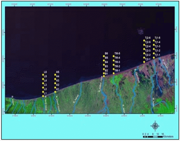
The field data used includes observational samples of chlorophyll-A concentrations collected on the east coast of the Caspian Sea, between the Lavijrood and Nekarood rivers in Mazandaran province. The field observations were planned and implemented at scheduled stations as shown in Fig. 1.
As shown, observations were made in 3 pairs of strips, with about 9 km between the strips in each pair. The stations in each strip are 3 km from each other and the distances between the first and second pair and the second and third pair are about 40 km and 25 km, respectively. The collected set of data has been provided below:
Table 1
Data Gathered from Field Data Sampling Stations [19]
Date
Station
Depth (m)
Chlorophyll-a (μg/L)
July 30, 2011
B1
1.09
1.44
B2
13.1
0.39
B3
23.6
0.33
B4
34
0.09
B5
73.7
0.39
TM-1
1.3
0.47
TM-2
16.6
0.29
TM-3
25
0.29
TM-4
34.1
0.31
TM-5
62.2
0.28
July 31, 2011
A1
1.3
0.8
A2
25.5
0.15
A3
37.8
0.28
A4
58.2
0.28
A5
98.09
0.21
L1
77
0.61
L2
51.4
0.29
L3
36.9
0.46
L4
51.4
0.3
L5
77
0.31
August 15, 2011
B1
3.2
0.8
B2
12.9
0.5
B3
23.9
0.4
B4
33.3
0.2
B5
63.3
0.2
TM-1
4.7
0.5
TM-2
16.3
0.2
TM-3
25.5
0.2
TM-4
34.3
0.3
TM-5
63.3
0.2
August 17, 2011
A1
2.2
0.7
A2
26.3
0.3
A3
37.2
0.5
A4
57.3
0.3
A5
98.15
0.3
L1
3.4
0.8
L2
25.6
0.3
L3
35.7
0.2
L4
51.4
0.4
L5
75.7
0.5
September 5, 2011
B1
3.2
1.2
B2
13.1
0.6
B3
23
0.3
B4
33.1
0.4
B5
63.1
0.7
TM-1
4.6
1.4
TM-2
16.3
0.4
TM-3
24.6
0.5
TM-4
33.5
0.4
TM-5
63.7
0.3
September 15, 2011
A1
1.52
3
A2
25.9
1.2
A3
37.2
0.8
A4
57.6
0.6
A5
97.7
0.4
L1
2.6
1.2
L2
25.6
1.2
L3
38.3
1
L4
51.2
0.6
L5
75.6
0.8
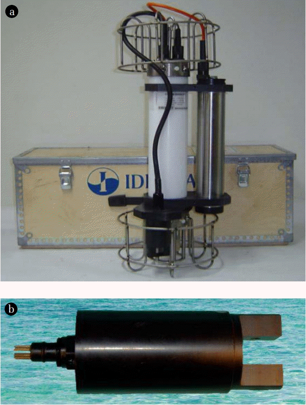
The samples were analyzed with a fluorometer mounted on a combined CTD monitor as shown in Fig. 2(a) in the supplementary materials. The monitor, “Ocean Seven 316 Probe” (IDRONAUT, Italy) measures the seawater’s physical parameters (electrical conductivity, temperature, and depth). Fig. 2(a) shows the device, which can be used to measure Chlorophyll-A concentration by installing a fluorometer sensor. The Sea point fluorometer used is shown in Fig. 2(b). It can determine the chlorophyll concentration to 0.1 μg/L precision by measuring the water’s fluorescence.
The samples were collected and observed at the approximate transit time of MODIS over the Caspian Sea on 20 d, yielding a total of 92 samples.
2.2. Satellite Data
MODIS is on the Aqua satellite. It orbits at 705 km and has a 55-degree viewing angle, giving a ground width of 2,330 km. It records the spectral range 400 nm to 14 um at high, 12-bit, resolution. It uses 36 spectral bands, of which 2 have a ground pixel size of 250 m, 5 a ground pixel size of 500 m, with 1 km pixel size for the other 29. The 250 and 500 m bands are designed for geological studies and cloud detection. The information from the 1 km bands, numbers 9, 10, 11 and 12, covering the 438 to 556 nm spectral range, are suitable for determining chlorophyll concentrations [20] and therefore, used in this study. Images from the Caspian Sea area were gathered from the MODIS site on the same day as field data were collected so that the two data sets could be compared.
3. Method
The MODIS images (MOD 02 1 km Level 1B Calibrated Radiance) gathered on the same day as the field data were adjusted with various radiometric pre-processes, including balancing performance between detectors, systematic geometric corrections. All geometric pre-processing was done with ENVI software, using the image’s side-information and the nearest neighbor in the sampling period during this study to minimize the error occurred due to the image processing. Fig. S1 in supplementary materials is a schematic showing the study methods used.
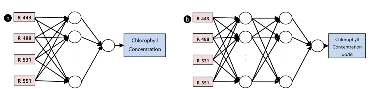
The field data were divided into training and evaluation categories. Evaluation data were used only to evaluate the accuracy of the results, while the training data were used in experimental algorithms and artificial multi-layer perceptron (MLP) NNs to estimate the chlorophyll-A concentration. Both Chlor-a-2 and Chlor-a-3 methods were among those that their use is very common. The structures of the two NNs used are shown in Fig. 3(a) and (b).
As shown in Fig. 3, the input layer introduces data from bands 9, 10, 11, and 12 as network inputs, and the output layer, a single neuron, gives the chlorophyll-A concentration (mg/L). The optimal number of neurons for the hidden layers was determined by trial and error, the number being increased gently to obtain the required result. The Levenberg-Marquardt algorithm (LM) as used to train the NN. LM is a combination of two Newton algorithms and a descending gradient that can establish a perfect balance between speeds of Newton’s method and ensure the convergence of the descending gradient method [21]. The activation functions used in the hidden layers are in the single-layer intermediate mode of the sigmoid tangent and consequently, in the two-layer model, it will become the sigmoid tangent of the first layer’s sigmoid tangent. Besides, the activation function of the NN’s output layer was considered as a linear one.
After estimating the concentration of chlorophyll-A, the estimated concentration is compared with the field data for evaluation and validation. The data allocated to validation were solely used for that purpose and excluded from others that used in network training step. The evaluation parameters, RMSE, mean relative error (MRE), and pearson correlation coefficient (R2) are defined by the relationships in Eq. (3), (4) and (5), respectively.
(3)
(4)
(5)
where and are, respectively, the measured and estimated values, and N the number of samples.
4. Results and Discussion
4.1. Implementation and Evaluation of Empirical Algorithms
As discussed in the methods Section, two algorithms were used in this study. To implement algorithms Chlor-a-2 and Chlor-a-3 initially, a number of observations were chosen randomly from different days, and the reflectivity of the 448, 551, and 488 nm wavelengths extracted from the MODIS images of the selected days and stations. The algorithms were then used to estimate the concentration of Chlorophyll-A at the stations. The estimations of accuracy parameters were also investigated for the algorithms – Table 2 shows the results.
As can be seen, the algorithms are not successful in determining the Chlorophyll-A content of Caspian Sea coastal waters.
4.2. Implementation and Evaluation of Artificial NNs
Some 83 samples were taken at random from the chlorophyll-A concentration field data, along with the 4-band radionuclide values – 60% for training, and 20% each for sample testing and internal evaluation. After the training step, 9 samples with suitable time and space distribution were used for validation, the generalization of the network, and network performance observation using the data that were not applied during the training step. In the training step, the initial weight values were selected randomly, and multiple trial and errors were implemented to find the best values. Also, because of the random selection of the training samples, we faced instability problem in analyzing and managing the network. In several consecutive implementations, the optimal response of each network was obtained and the differences between these responses were evaluated, afterward.
For a better assessment, the Standard deviation (SD) of the evaluation parameters represents the network response stability. Obviously, the higher the evaluation parameter SD, the more stable the network. The evaluation parameter mean represents the network’s general performance.
4.2.1. Neural network with one hidden layer
The number of neurons was varied from 5 to 25 in a NN with a single hidden layer to evaluate the effect of the network’s structure on its results and stability. It was comprehended that increasing the number of neurons to 15 improves the general accuracy of the response. Increasing the number beyond 15, however, produced a relative decrease in the response accuracy and this, possibly, have occurred because insufficient training samples were used. On the other hand, when fewer than 15 neurons are used, the network’s response accuracy is poorer owing to the fact that the network is not smart enough – see Fig. 4.
The NN with 15 neurons in the hidden layer reported an SD (RMSE) of 0.013 and a mean (RMSE) of 0.108. These were the best values for any single-layer network. R2, however, was, which is relatively low and indicates a low correlation between the actual and expected network outputs.
4.2.2. Neural network with two hidden layers
The number of neurons in an NN with two hidden layers was varied from 5 to 15 neurons for each layer was tested. If there were 5, 10 or 15 neurons in the first layer, the best results were obtained for the 5th, 10th and 10th neurons in the hidden layer. Fig. 5 is a comparison between the best results from two-layer NNs (5, 5), (10, 10) and (15, 10).
Of the two-layer structures, with 5 neurons in each of the first and second hidden layers, resulting in the best in terms of accuracy and stability. The best response from a structure with two hidden layers had an RMSE = 0.064. Comparing to the results from the best single-layer NN (15 neurons in the hidden layer) indicates that, the two network types are almost the same on the basis of accuracy, the correlation of responses with the actual results (R2) is higher for the two-layer network, though. Generally, in NNs with two hidden layers, the average R2 is about 0.5 (unacceptable for model efficiency) – i.e., there is a higher correlation with the expected responses than for a single-layer network, with an average R2 of about 0.36.
4.2.3. Evaluation of the effect of training sample numbers
As noted, about 50 field samples were used for network training in the study. The cost of collecting field samples is high and there are considerable performance problems, so using enough data for the training step is of high importance. Consequently, the effect of the number of training samples on the optimal networks was investigated – see Table 3.
As shown in Table 3, the NN with one hidden layer and 15 neurons requires at least 34 training samples to maintain its optimal response level. The NN with two hidden layers and 5.5 neurons resists reductions in training sample numbers, and even with only 20 can maintain an acceptable accuracy level. Fig. S2 which provided in the supplementary materials, shows the distribution of chlorophyll-A in the Caspian Sea on July 27, 2011, with the optimal dual-layer NN output on MODIS images.
The ribbon strips in Fig. S2 arise from an error in the MODIS images, a problem that can be resolved. However, a generalization of the results to all areas of the Caspian Sea is not possible and requires wider geographical field sampling. However, what is obtained in Fig. S2 as the optimal neural network output is consistent with the results of the research on chlorophyll-A in the Caspian Sea, which indicates the ability of this neural network to estimate chlorophyll-A concentrations. Due to the counterclockwise rotation of the water in the Caspian Sea, which transfers water with high nutrient and phytoplankton content from the northern to the western zones, the Chlorophyll-A concentration is higher along the sea’s western coast than in the eastern regions.
5. Concluding Remarks
The experimental algorithms used do not make useful estimates of chlorophyll-A concentrations in coastal areas of the Caspian Sea. Chlor-a-2 and Chlor-a-3 resulted RMSE = 0.47 μg/L and RMSE = 0.79 μg/L, respectively – i.e., Chlor-a-3 was better but their precision are inadequate after all.
In networks with one hidden layer, the network with 15 neurons is most accurate and in networks with two hidden layers (5, 5) neurons is the best. Both the single and two hidden layer networks achieved RMSEs of about 0.1 μg/L under good conditions. As the accuracy of the field data used to train the networks was also about 0.1 μg/L, it is clear that both types of NN are suitable for use estimating chlorophyll-A concentrations in the Caspian Sea from MODIS sensor data.
considering the value of 0.5 / lit for chlorophyll-A, the relative tolerance of the neural network response, which is obtained by dividing RMSE = 0.1 by 0.5, is estimated to be about 20%. In other words, the accuracy of this network can be 80%. Due to the relative accuracy of field observations in the same range, this is the highest expectation that we can use the neural network to estimate the chlorophyll-A content in terms of training data. Comparison of the single- and two-layer NNs shows that, while their accuracies are almost the same, the mean value of R2 in the two-layer network is the better of the two. Single-layer networks are slightly better than those with two layers, however. On the other hand, the network with two layers needed less training (fewer samples) than the single-layer one, to achieve about 0.1 μg/L precision, matching the training samples’ accuracy.
The study showed that the optimal NN for estimating chlorophyll-A concentrations from MODIS images in Caspian Sea coastal areas is one with two hidden, 5 neuron layers. It has an RMSE of 0.064 μg/L with a correlation coefficient of about 50% in the best situations.
1. Jensen JR. Remote sensing of the environment: An earth resource perspective. 2nd edUniv of South Carolina: Pearson Prentice Hall; 2007. p. 409–440.
2. Tang D, Kawamura H, Lee M, Dien TV. Seasonal and Spatial Distribution of Chlorophyll a Concentrations and Water Conditions in the Gulf of Tonkin, South China Sea. Remote Sens Environ. 2003;85:475–483.
3. Gregg WW, Casey NW. Global and regional evaluation of the seaWiFS Chlorophyll data set. Remote Sens Environ. 2004;93:463–479.
4. Pinkerton MH, Richardson KM, Boyd PW, et al. Intercomparison of ocean colour band-ratio algorithms for Chlorophyll concentration in the subtropical front East of New Zealand. Remote Sens Environ. 2005;97:382–402.
5. Allan MG, Hamilton DP, Hicks BJ, Brabyn L. Landsat remote sensing of chlorophyll a concentration in central North Island lakes of New Zealand. Int J Remote Sens. 2011;32:2037–2055.
6. O’Reilly JE. Ocean Color Chlorophyll Algorithms for SeaWiFS, OC2, and OC4: Version 4. Hooker SB, Firestone ER, editorsSea WiFS Postlaunch Calibration and Validation Analyses, Part 3. Washington D.C.: NASA Technical Memorandum; 2000. p. 9–11.
7. Carder K, Chen F, Lee Z, Hawes S, Cannizzaro J. Modis ocean science team algorithm theoretical basis document, Case 2 Chlorophyll a [Internet]. Available From: http://modis.gsfc.nasa.gov/data/atbd/atbd_mod19.pdf
8. Miles TN, He R. Temporal and spatial variability of Chl-a and SST on the South Atlantic Bight: Revisiting with cloud-free reconstructions of MODIS satellite imagery. Cont Shelf Res. 2010;30:1951–1962.
9. Kavak MT, Karadogan S. The relationship between sea surface temperature and chlorophyll concentration of phytoplankton in the Black Sea using remote sensing techniques. J Environ Biol. 2012;32:493–498.
10. Hu C, Chen Z, Clayton T, Swarzenski P, Brock J, Muller-Karager F. Assessment of estuarine water-quality indicators using MODIS medium Resolution bands: Initial results from Tampa Bay. Remote Sens Environ. 2004;93:423–441.
11. Hornik K, Stinchcombe M, White H. Multilayer feedforward networks are universal approximators. Neural Netw. 1989;2:359–366.
12. Parlos AG, Chong KT, Atiya AF. Application of the recurrent multilayer perceptron in modeling complex process dynamics. Neural Netw. 1994;5:255–266.
13. Lippmann RP. An introduction to computing with neural networks. IEEE ASSP Magazine. 1987;4–22.
14. Looney CG. Pattern recognition using neural networks: Theory and algorithms for engineers and scientists. Oxford: Oxford Univ. Press; 1997.
15. Holyer R, Sandidge J. Coastal bathymetry from hyperspectral observation of water radiance. Appl Optics. 1998;65:341–345.
16. Lee Z, Zhang M, Carder K, Hall L. A neural network approach to deriving optical properties and depths of shallow waters. Proceedings, Ocean Optics XIV. Ackleson SG, Campbell J, editorsWashington D.C.: Office of Naval Research; 1998.
17. Kishino M, Tanaka A, Ishizaka J. Retrieval of Chlorophyll a, suspended solids, and colored dissolved organic matter in Tokyo Bay using ASTER data. Remote Sens Environ. 2005;99:66–74.
18. Doerffer R, Schiller H. The MERIS Case 2 water algorithm. Int J Remote Sens. 2007;28:517–535.
19. Gholamalifard M. Satellite monitoring of optically active components of Caspian Sea by inverse modeling of radiative transfer equation [dissertation]. Tehran: Tarbiat Modares Univ.; 2013.
20. Martin S. An introduction to ocean remote sensing. Cambridge: Cambridge Univ. Press; 2004. p. 426.
21. Hagan MT, Menhaj MB. Training feedforward networks with the marquardt algorithm. IEEE Trans Neural Netw. 1994;5:989–993.
Fig. 1
Field data sampling stations.
Fig. 2
(a) CTD device, (b) Sea point fluorometer sensor mounted on the CTD device.
Fig. 3
Structures-(a) Three-layer NN; and (b) Four-layer NN.
Fig. 4
NN with a single hidden layer.
Fig. 5
Comparison of the best networks with two hidden layers.