Analysis of drought in northwestern Bangladesh using standardized precipitation index and its relation to Southern oscillation index

Article information

Environmental Engineering Research. 2016;21(1):58-68

Publication date (electronic) : 2015 December 16

doi : https://doi.org/10.4491/eer.2015.115

Department of Civil and Environmental Engineering, Shahjalal University of Science and Technology, Sylhet 3114, Bangladesh

^†Corresponding author: Email: k.hasancee@gmail.com, Tel: +880-821-713491 Fax: +880-821-715257

Received 2015 October 01; Accepted 2015 December 14.

Abstract

The study explored droughts using the Standardized Precipitation Index (SPI) in the northwestern region of Bangladesh, which is the drought prone area. In order to assess the trend and variability of monthly rainfall, as well as 3-month scale SPI, non-parametric Mann-Kendall (MK) tests and continuous wavelet transform were used respectively. The effect of climatic parameters on the drought in this region was also evaluated using SPI, with the Southern Oscilation Index (SOI) by means of the wavelet coherence technique, a relatively new and powerful tool for describing processes. The MK test showed no statistically significant monthly rainfall trends in the selected stations, whereas the seasonal MK test showed a declining rainfall trend in Bogra, Ishurdi, Rangpur and Sayedpur stations respectively. Sen’s slope of six stations also provided a decreasing rainfall trend. The trend of the SPI, as well as Sen’s slope indicated an increasing dryness trend in this area. Dominant periodicity of 3-month scale SPI at 8 to 16 months, 16 to 32 months, and 32 to 64 months were observed in the study area. The outcomes from this study contribute to hydrologists to establish strategies, priorities and proper use of water resources.

Keywords: Drought; Mann-Kendall test; Rainfall; SPI; Sen’s slope; Wavelet coherence; Wavelet power spectrum

1. Introduction

Drought is a hazard that affects the most people among all natural disasters, and yet it is the least understood and most complicated [1]. In Bangladesh, it is the most serious issue because of geographical location, high population density, high levels of poverty, and the reliance of many livelihoods on climate sensitive sectors, such as agriculture and fisheries [2]. It is a gradually developing occurrence that indirectly affects many lives. Continuous period of dry weather along with abnormal insufficient rainfall are the main cause of drought. It also occurs when evaporation and transpiration exceed the amount of rainfall for a reasonable period.

Rainfall is the primary factor governing the development and persistence of the drought phenomenon [55]. Therefore, the assessment of patterns and trends of rainfall was conducted in this study. Trend analysis was carried out using a non-parametric MK test. It is a widely used test [3–12] for its suitability for non-normally distributed data and censored data. The continuous wavelet transform is an important tool to study variations of variables like rainfall [13–20]. Trend and variation analysis of rainfall by adopting MK test and wavelet power spectrum respectively, are rare studies in Bangladesh, though some other methods were applied for this analysis.

McKee et al. [21] developed the SPI in order to observe and describe drought. The probability of rainfall within a specific time period is measured, and then transformed into an index table, on which the SPI is based. Several countries, including Turkey, Argentina, Canada, Spain, Korea, Hungary, China and India, have used this instrument in order to monitor droughts in real-time and analyze the conditions that led to the drought [22–28]. Keka et al. [56] analyzed the drought in the eastern part of Bangladesh. Yearly drought analysis was performed by three climatic indices. The climatic indices are De Mortone Aridity Index (IdM), Seleaninov Hydrothermic Index (IhS), and Donciu Climate Index (IcD). Jahangir et al. [57] used SPI to evaluate the precipitation deficit, and Markov chain model was used to quantify the drought in agricultural extent.

SPI results from transforming normal quantile into the fitted parametric distribution of the original value. SPI is used to assign a single numeric value to the rainfall that can be compared across a region’s noticeably different climates. Utilization of the index helps to determine the infrequency of a current drought because of the SPI standardization. SPI can be used to perform quantitative analysis concerning changes in precipitation when compared to overall climatic means. For example, summer precipitation dominates annual precipitation, thereby, overriding the effects of small precipitation variability throughout the year, may inhibit drought in the short-term, but has very little long-term effect. Furthermore, SPI can identify types of drought by using different time scales [21, 29]. The SPI could be calculated for a 3-month, 6-month, 12-month period, etc. According to Mishra and Desai [31], 2–3 months period of SPI may indicate agricultural drought best. It also reflects short-term moisture conditions of soil. In Bangladesh, drought is defined as the period when the moisture content of soil is less than the required amount for crop growth during the normal crop-growing season. Moreover, the economy of Bangladesh largely depends on agriculture. Therefore, 3-month scale SPI was used to conduct this study.

When exploring the cause of droughts, a climatic index may be provided by a coupled atmosphere-ocean system, which may be used to control precipitation. For example, the El Nio-Southern Oscillation (ENSO) phenomenon, which took place in the tropical Pacific, impacted areas beyond the tropical regions with hydro-meteorological disasters like floods and droughts [30]. The other factors affect drought are sea surface temperature, deforestation, over exploitation of resources, rising level of CO₂ and green house gases etc. [58].

The present study aimed to analyze the trend and pattern of rainfall to see the transient variations, as well as investigate the drought phenomena using the SPI in northwestern Bangladesh. It also focused on the analysis of SPI using wavelet transform. Linkage was sought between the SPI and the climate indices, like SOI, by means of wavelet coherence.

2. Materials and Methods

The study area is northwestern part of Bangladesh, which is a hard-hit region among drought-prone areas in Bangladesh [62]. Monthly rainfall data, collected by the Bangladesh Meteorological Department (BMD), was used in the study. The required SOI data set was collected from the National Oceanic and Atmospheric Administration (NOAA). Details of the rainfall stations and data length are given in Table 1. The locations of the stations are shown in Fig. 1. Statistical trend analysis and wavelet analysis was carried out using the MINITAB and MATLAB respectively.

Table 1

Location of Stations

Fig. 1

Study area.

2.1. Calculation of SPI

In order to calculate the SPI in a specific location, the precipitation record for a long-term period of time is collected, and this data is fitted to a probability distribution and then converted into a normal distribution. Estimating the SPI involves describing frequency distribution of precipitation using a gamma probability density function:

(1) f(x)=xα-1βαΓ(α)e(-x/β)

where, is precipitation amount ( > 0), α (α > 0) & β (β > 0) are continuous shape parameter. In Eq. (1), Γ(α) is the gamma function. The parameters α and β can be estimated using the maximum likelihood method as [32]:

(2) α=14A(1+1+4A3)

(3) β=x¯α

where,

(4) A=ln (x¯)=∑ln (x)n

where, n is number of precipitation observations and χ̄ is average precipitation amount.

The estimated parameters will be used to derive the cumulative probability of observed precipitation values for the given month and time scale (e.g. 3 months) over each pixel

(5) f(x)=∫0xg(x)dx=1βαΓ(α)∫0xxα-1 e-x/β dx

f, t = x/β then equation 5 becomes the incomplete gamma function:

(6) f(x)1Γ(α)∫0xtα-1 e-t dt

It is possible to have several zero values in a sample set. In order to account for the zero value, probability, since the gamma distribution is undefined for x = 0, the cumulative probability function for gamma distribution is modified as:

(7) H(x)=q=(1-q)G(x)

here, q and (1–q) denote the probabilities of zero and nonzero precipitations, respectively. The SPI is then derived from the cumulative probability.

(8) Z=SPI=-(t-c0+c1t+c2t21+d1t+d2t2+d3t3) for 0<H(x)≤0.5

(9) Z=SPI=+(t-c0+c1t+c2t21+d1t+d2t2+d3t3) for 0.5<H(x)≤1

Here,

(10) t=ln(1(H(x))2) for 0<H(x)≤0.5

(11) t=ln(1(1.0-H(x))2) for 0.5<H(x)≤1

where, c₀, c₁, c₂, d₁, d₂ and d₃ are constant value.

Hence, the SPI represents a Z-score variable. At a given time, the SPI may be computed for different time scales, say one month or longer, by computing the cumulative probability at a given location for the time scale selected. Usually, 3, 6, 9, 12 and 24-month time scales are considered to give information about drought and its impacts on different segments of the hydrological cycle in the area. SPI timescale intervals shorter than 1-month and longer than 24-months may be unreliable [33]. Classification based on SPI values is shown in Table 2 [34].

Table 2

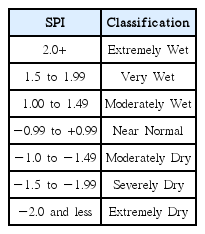
Classification of SPI Values

2.2. Mann-Kendall

The original MK test [35–36] assumed that the time series had no seasonal pattern. Later on, Hirsch et al. [37] developed an extension of the MK test to allow for seasonal variations as they are existent in most hydro-meteorological time series. The hypothesis of the MK trend test is:

H_O (Null Hypothesis): Time series values are independent and identically distributed, i.e. there is no trend.
H_A (Alternative Hypothesis): There is a monotonic (not necessarily linear) trend.

In this two-tailed test, the differences between two different time scales of measured data are analyzed using the MK trend test. Earlier-measured data values are compared to later-measured data values, and where n is the total number of observations, the result is n(n-1)/2 possible pairs of data. The test statistic S is given as follows:

(12) S=∑k=1n-1∑j=k+1nsin (xj-xk)

where

(13) sin (xj-xi)={+1,>(xj-xi)0,=(xj-xi)-1,<(xj-xi)

where, x_j and x are the annual values for years j and i, respectively, and j>i.

Thus, a large positive value of S indicates a strong positive (increasing) trend while a large negative value of S implies a negative (decreasing) trend. The non-parametric assumption of MK test for a time series with a large number of values, is documented to allow the use of a regular Z-test to determine whether or not a trend is significant [38]:

(14) Z={s-1n(n-1)(2n+5)-∑j=1qtj(tj-1)(2t+5)18s>10s=0s+1n(n-1)(2n+5)-∑j=1qtj(tj-1)(2t+5)18s<1

where, n is sample size; q is number of tied groups in the data set and t_j is number of data points in the j^th tied group.

Z follows standard normal distribution with mean zero and variance unity.

2.3. Seasonal Mann-Kendall Test

The seasonal MK trend test avoids the shortcomings of the regular MK test in the presence of seasonal data. Hirsch et al. [37] developed this test, which consists mainly of computing the regular MK test separately for each season (here month) and combining the results to get Kendall’s test statistic. Of course, depending on the nature of the time series, a season could be a month or a quarter of a year, a year or any combination of these. So for monthly “seasons”, January data are compared only with January, February only with February, etc., so that, overall, there are m=12 seasons. No comparisons are made across season boundaries.

Here, S′ is the sum of Kendall’s S, computed as discussed in the previous section for each season g.

(15) S′=∑g=1mSg

2.4. Sen’s Slope

The Sen’s Slope method [39] is used to estimate the extent of the trend by calculating the slope as a change in measurement over time. It was used in this study because it can be considered as a method that provides strong estimation of the trend [40].

(16) Q′=xt′-xtt′-t

where, Q′ is slope between data points x_t_′ and x_t;x_t_′ is data measurement at time t′ and x_t is data measurement at time t. Sen’s estimator of slope is simply given by,

(17) Q=Q′[N+12] if N is odd

(18) Q=12(Q′[N+12]+Q′[n+22]) if N is even

where, N is the number of calculated slopes. Throughout this study, a significance-level of 0.05 is used for analysis indicating 95% confidence.

2.5. Southern Oscillation Index (SOI)

The SOI is an index that is based on the difference in air pressure between Darwin and Tahiti. The SOI is closely related to the El Nio and La Nia climate phenomenon. A consistently negative SOI often indicates the presence of an El Nio. However, a consistently positive SOI often indicates the presence of a La Nia. The study of the EI Nino-Southern Oscillation (ENSO) phenomenon is critical because hydro-meteorological disasters, like floods and droughts, can occur beyond the tropical region as a result of its presence in the tropical Pacific [30]. The SOI is usually computed on a monthly basis with values over longer periods, such a year, being sometimes used. It is calculated as follows:

(19) SOI=10×[Pdiff-Pdiffav]SD(Pdiff)

where, P_diff is the difference between sea level pressure [(average Tahiti mean sea level pressure for the month) - (average Darwin mean sea level pressure for the month)], P_diffav is long term average of P_diff for the month in question, and SD(P_diff) is long term standard deviation of P_diff for the month in question.

The El Nio phenomenon is associated with higher SSTs in the central and eastern tropical Pacific Ocean and less strong Pacific Trade winds. The El Niño phenomenon generally corresponds to a decrease in rainfall. The La Niña phenomenon is the reciprocal to the El Niño phenomenon and brings above normal rainfall.

2.6. Wavelet Analysis

The time domain and the frequency domain make up a time series, which is analyzed by the wavelet transform, when it contains many different frequencies of non-stationary power [41]. Simultaneously converting a one-dimensional time series into a diffused two-dimensional time-frequency image allows for a signal analysis of a localized time and frequency, which is maintained by the wavelet analysis. Using wavelet transforms to analyze time series is a rather modern process. Wavelet transforms can be used to describe processes that occur over finite, spatial, and temporal domains, as well as multiscale and nonstationary processes [42], similar to the Fourier transform (STFT). In the traditional Fourier transform (FT), a signal is split into a series of sine waves of different frequencies. However, the signal is split into wavelets, which are transformed from the original wavelet, when using the wavelet transform. Further, the signal is provided in a time scale presentation in the wavelet analysis, but only the spectral components within a signal are identified using the Fourier spectral analysis. Variances of time and amplitudes compared to frequency can be shown by changing the wavelet time scale and converting the versions of the wavelet to a graph, using the wavelet analysis [19]. Therefore, wavelet analysis is an appropriate, strong, and useful tool for identifying trends, shifts, breakdown points and discontinuities [13, 18] and analyzing the statistical properties of these time series.

Recently CWT has been used for analyzing climate variability and the temporal variability of rainfall and runoff [13, 18, 19, 42–48]. Mathematically CWT can be expressed as follows [49]:

(20) C(a,b)=1a∫s(t) Ψ(t-ba)dt

where C is the wavelet coefficient, a and b are scale and position functions respectively, s(t) is the signal (SPI and SOI in this study) and Ψ is the wavelet function. The wavelet coefficients (C) are the result of the CWT of signal s(t). The Morlet wavelet has been used in this study.

2.7. Wavelet Coherence

Time and frequency can by analyzed simultaneously when comparing the strength of the relationship between two time series, as identified by the wavelet coherence analysis. Variances over time, when two time series are significantly coherent, can be identified and analyzed.

Following Torrence and Webster [50] the wavelet coherence of two time series x and y is:

(21) WTC=S(Cx*(a, b) Cy(a, b))S(∣Cx(a, b)∣2) S(∣Cy(a, b)∣2)

where C_x(a, b) and C_y(a, b) denote the continuous wavelet transforms of x and y at scales a and positions b. The superscript * is the complex conjugate and S is a smoothing operator in time and scale.

3. Results and Discussion

Wavelet analysis was chosen to identify the hidden periodicity of rainfall because the standard Fourier transform analysis will be applied, if it has stationarity and the aggregate of variable periodic components for the entire interval. Both requirements must be fulfilled, and most time series in hydrology and meteorology do not meet the conditions. However, rainfall patterns at varying timescales and periods can possible identified using wavelet transform.

Fig. 2 shows continuous wavelet transform to find the relative power of monthly rainfall at different period scales from the year 1983 to 2012 in the Bogra, Dinajpur, Ishurdi, Rajshahi, Rangpur and Sayedpur stations respectively. The thick, curved black line in wavelet power spectrum represents the cone of influence (COI), where zero padding reduced the variance. The dashed line is the 5% significance level for the global wavelet spectrum. A dominating periodicity between 8 and 16 months from 1983 to 2012, as well as a significant peak above the 95% confidence level in the global wavelet spectrum, were observed in the corresponding situations. There is no strong wavelet power spectrum among other periods. However, transient rainfall variation was noticed in the normalized monthly rainfall time series. To see the trend of rainfall, the MK test was conducted. In the present study, we used the pre-whitening approach for removing autocorrelation effects. Then the MK test was applied to the blended series to assess the significance of the trend.

Fig. 2

Wavelet analysis of monthly rainfall at (a) Bogra, (b) Dinajpur, (c) Ishurdi, (d) Rajshahi (e), Rangpur, and (f) Sayedpur. Normalized monthly rainfall, wavelet power spectrum and global wavelet spectrum are shown in (A), (B) and (C) respectively. The thick curved black line in wavelet power spectrum represents the cone of influence (COI). The dashed line in global wavelet spectrum shows the 95% confidence level. The strength of power (%) in the contour image in wavelet power spectrum is labelled by color (right corner).

MK Statistics and the corresponding p-value at 5% significance level of monthly rainfall between 1983 and 2012 are shown in Table 3. Table 3 indicates the p-value is higher than the significance level (0.05). So the null hypothesis was accepted. It should be noted that if null hypothesis is accepted, in some cases, that doesn’t mean that it was proven that there is no trend; rather, it is a statement that the evidence available is not sufficient to conclude that there is not a trend [51].

Table 3

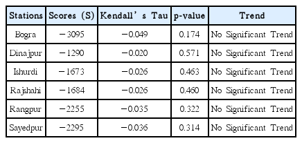
Mann-Kendall Test Results of Monthly Rainfall

The results of seasonal MK test for monthly rainfall between 1983 and 2012 are shown in Table 4. The trend test result showed a decreasing trend of monthly rainfall in Bogra, Ishurdi Rangpur and Sayedpur stations, whereas statistically no significant trend in Dinajpur and Rajshahi respectively. However, Rahman & Begum [60] studied trends of rainfall of island Bhola in Bangladesh using MK test. They found rising rates of precipitation in some months and decreasing trend in some other months obtained by these statistical tests suggesting overall insignificant changes in the area. Hasan et al. [61] assessed rainfall of southeast Bangladesh using MK test. This study indicated amount of annual rainfall is increasing although this trend is not statistically significant.

Table 4

Seasonal Mann-Kendall Test Results of Monthly Rainfall

Fig. 3 illustrates Sen’s slope of monthly rainfall for different stations. Sen’s slope was low (−0.014) at Bogra and high (−0.001) at Dinajpur stations respectively. Sen’s slopes at different stations were negative, indicating a decline in rainfall. This might have affected the drought phenomena in this region.

Fig. 3

Sen’s Slope of monthly rainfall for different stations.

SPI values of 3-month scale from 1983 to 2012 at different selected stations in the northwestern Bangladesh are shown in Fig. 4. Data showed the presence of alternative dry and wet periods, but with no regular annual shifts. According to SPI, Bogra was affected by extremely dry conditions in the years 1999, 2006 and 2011 as well as extremely wet conditions in the years of 1986, 1988, 1992, 1998, 2000, 2003 and 2005 respectively. The driest period was noticeable in the years 1992, 1994, 1995, 2001, 2006 and 2011 while an extremely wet state was clear in the years 1987, 2002 and 2005 in Dinajpur respectively. Ishurdi had extremely dry events in the years 1994, 1999, 2003 and 2011 whereas extremely wet events in the years 1990, 1992 and 2005 respectively. Rajshahi was confronted by extremely dry events in the years 1992, 1999 and 2010 including extremely wet events in the years 1983, 1990, 1992 and 1997 respectively. Extreme dry periods were visible in the years 1994, 1995, 2000 and 2011 whereas extreme wet periods were in the years 1984, 1987, 1996 and 2002 respectively in Rangpur. However, at Sayedpur extreme drought events occurred in the years 1992, 1994, 1995, 2000, 2008 and 2011 while extreme wet events happened in the years 1987, 1996, 1998, 2001, 2002 and 2003 respectively. According to the historical data, the most devastating drought episodes occurred in 1994 throughout the country [52]. This drought was clearly identified by the SPI in Dinajpur, Ishurdi, Rangpur and Sayedpur respectively. The flood event of 1998 [53] was detected by SPI in Bogra and Sayedpur, too. It was observed that Dinajpur, Ishurdi and Sayedpur were more drought prone area in the study region.

Fig. 4

SPI values of 3-month scale from 1983 to 2012 at (a) Bogra station, (b) Dinajpur station, (c) Ishurdi station, (d) Rajshahi station, (e) Rangpur station, (f) Sayedpur station.

MK statistics and their corresponding p-value at 5% significance level for 3-month scale SPI between 1983 and 2012 are shown in Table 5. Table 5 indicates the p-value is lower than the significance level (0.05). So the null hypothesis was rejected. High negative values of the score for MK test referred to a decreasing trend in all stations.

Table 5

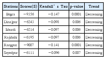
Mann-Kendall Test Results for 3 Month Scale SPI

The results of seasonal MK test for 3-month scale SPI between 1983 and 2012, which accounted seasonal time series (i.e., 12-months) are provided in Table 6. The trend test result showed that among the six stations, only Bogra and Rangpur showed the presence of a statistically significant decreasing trend in the three situations.

Table 6

Seasonal Mann-Kendall Test Results for 3 Month Scale SPI

Fig. 5 presents Sen’s slope of 3-month scale SPI for different stations. Sen’s slope was low (−0.002) at Bogra, and Rangpur stations while high (−0.001) at Dinajpur, Ishurdi, Rajshahi and Sayedpur stations respectively. Sen’s slopes at different stations were negative, indicating that there was a trend towards increasing dryness in the region. This might have affected water demand and put additional pressure on already scarce water resources.

Fig. 5

Sen’s Slope of 3-month scale SPI for different stations.

In order to observe the variability of SPI along the study region, continuous wavelet power spectrum (WPS) was evaluated. In addition to this, continuous wavelet transform was conducted to identify the relative power of SPI in different period scales. It was conducted using Morlet wavelet transforms.

Fig. 6(a–f) provides continuous wavelet power spectrum of 3-month scale SPI at Bogra, Dinajpur, Ishurdi, Rajshahi, Rangpur and Sayedpur stations respectively. SPI showed a significant variability between 16 to 32 months period between the years 1987 and 2010 in Bogra. However, the peak above the 95% confidence level was observed at 8-month period in the global wavelet spectrum. Strong power existed for the 32 to 64 months period (1/16 to 1/32 frequencies) between 1983 and 2007 in Dinajpur. A higher concentration of the power spectrum was noticed for the periods 16 to 32 during 1991 to 2004, whereas the peak global spectrum exceeded the dashed line at 8–16 months period at Ishurdi station. The dominant periodicities existed from 16 to 32 months during 1990 to 1995, although significant peak existed between 8 and 16 months in the global wavelet spectrum in Rajshahi. A strong wavelet power spectrum was also observed for the 32 to 64 months period between 1983 and 2007, as well as the peak global wavelet spectrum touched the dashed line at 5% significant level in Rangpur station. 8 to 16 months and 32 to 64 months significant variability during 1991 to 2000 and 1984 to 2004 was also found in Sayedpur station respectively. Here, peak passed the dashed line at 8 to 16 months period in the global wavelet spectrum. Overall, periodicity of 3 month scale SPI at 8 to 16 months, 16 to 32 months and 32 to 64 months were significant in the selected stations.

Fig. 6

Wavelet analysis of 3-month scale SPI at (a) Bogra, (b) Dinajpur, (c) Ishurdi, (d) Rajshahi, (e) Rangpur, and (f) Sayedpur. The thick curved black line in wavelet power spectrum represents the cone of influence (COI). The dashed line in global wavelet spectrum shows the 95% confidence level. The strength of power (%) in the contour image in wavelet power spectrum is labelled by color (right corner).

SOI represents coupled atmosphere-ocean phenomena having huge impacts on hydroclimatology around the globe [54]. Therefore, the relationship between the SOI and 3-month scale SPI was evaluated by wavelet coherence. Wavelet coherency is useful to quantify the degree of relationship between two non-stationary series in the time frequency domain. If the phase arrows point rightward, the time series are in-phase and if left, the series are in anti-phase.

Fig. 7 shows wavelet coherency between SOI and 3-month scale SPI at Bogra, Dinajpur, Ishurdi, Rajshahi, Rangpur and Sayedpur stations respectively. This showed that SOI had significant coherency with the 3-month SPI between 4 and 8 month period from 1993 to 1998 in Bogra station. In Dinajpur, SOI had influence on 3-month SPI during 1990 to 1992 and 2005 at 4 to 8 months period. The 8 to 16 months and 32 to 64 months significant periodic coherency was observed for Ishurdi station over the period 1993–1994 and 1995–2000 respectively. In Rajshahi station, SOI showed significant influence on 3 month SPI at 4 to 8 months and 8 to 16 months period for the years 1994–1995. Rangour station had significant association between SOI and 3 month SPI for 4 to 8 months and 8 to 16 months period during 1991 to 1994 and 2005 respectively. Dominating influence of SOI on 3 month SPI was noticed at 4 to 8 months, 8 to 16 months and 32 to 64 months period during 1995 to 1996, 2005 and 1995 to 2004 in Sayedpur station respectively. So it was seen that significant wavelet coherence observed between SOI and 3 month SPI at 4 to 8 months, 8 to 16 months and 32 to 64 months periodicity, as well as short time span respectively. At all selected stations, during significant periods both extreme dry and wet conditions occurred. Thus, under a statistical point of view, a drought event could be influenced by SOI in this region. This condition seems to agree with previous study that variation of precipitation over central south-west Asia (Bangladesh, India, Pakistan etc.) is associated with variation of SOI [59]. So, this study suggests that a drought event could be influenced by SOI and it has importance for agriculture, as extreme dry and wet events occurred in this region several times.

Fig. 7

Wavelet coherency between SOI and 3-month SPI at (a) Bogra, (b) Dinajpur, (c) Ishurdi, (d) Rajshahi, (e) Rangpur, (f) Sayedpur stations. The thick black contour represents the 95% confidence level. The phase relationship is shown by arrows. Right and left arrows indicate an in-phase and anti - phase relationship respectively.

4. Conclusions

This study assessed rainfall pattern using MK test and wavelet power spectrum. Drought occurrence and its trend were analyzed by means of SPI and MK statistics respectively. It also evaluated the significant variability of 3-month scale SPI by wavelet power spectrum. Moreover, the relationship between SOI and SPI studied in the northwestern Bangladesh using wavelet coherence technique. A decreasing trend of monthly rainfall was found from the seasonal MK test in Bogra, Ishurdi Rangpur and Sayedpur stations respectively. Sen’s slope of six stations (−0.014, −0.001,−0.003,−0.004,−0.009 and −0.008 at Bogra, Dinajpur, Ishurdi, Rajshahi, Rangpur and Sayedpur respectively) showed also a declining pattern of monthly rainfall. Trend of SPI showed increasing dryness in this region. This might be the effect of rainfall variations. Dominant periodicity of 3-month scale SPI at 8 to 16 months, 16 to 32 months and 32 to 64 months were found in the selected stations. Although the coherency at selected stations were not significant for the entire study period, it was found that SOI influenced 3-month scale SPI at short time span.

In this work, we tried to relate drought to climatic parameters. However, droughts do not development singly from climactic phenomenon. Droughts are influenced by local geography, orography, soil parameter and vegetation, and these factors affect its development and localized severity. Therefore, understanding, predicting, and alleviating drought conditions should be the result of collecting the entirety of regional environmental information.

Acknowledgements

The author would like to thank BMD (Bangladesh Meteorological Department) for the support provided during this study. Wavelet package was provided by C. Torrence and G. Compo, and is available at URL: http://atoc.colorado.edu/research/wavelets/

References

1. Wilhite DA. Drought: A global assessment Hazards and disasters: A series of definitive major works 7th edth ed. London: Routledge Publishers; 2000.

2. Climate Change Cell. Department of Environment, Ministry of Environment and Forests, Bangladesh [Internet] c2009. [cited 2014 Dec 21]. Available from: http://www.climatechange-cell-bd.org/.

3. Hamed KH. Trend detection in hydrologic data: The Mann–Kendall trend test under the scaling hypothesis. J Hydrol 2008;349:350–363.

4. Zhang Q, Xu CY, Zhang Z, Chen YD, Liu CL. Spatial and temporal variability of precipitation over China, 1951–2005. Theor Appl Climatol 2008;95:53–68.

5. Kizza M, Rodhe A, Xu CY, Ntale HK, Halldin S. Temporal rainfall variability in the Lake Victoria Basin in East Africa during the twentieth century. Theor Appl Climatol 2009;98:119–135.

6. Lima MIP, Carvalho SCP, Lima JLMP, Coelho MFES. Trends in precipitation: analysis of long annual and monthly time series from mainland Portugal. Adv Geosci 2010;25:155–160.

7. Ngongondo C, Xu CY, Gottschalk L, Alemaw B. Evaluation of spatial and temporal characteristics of rainfall in Malawi: a case of data scarce region. Theor Appl Climatol 2011;106:79–83.

8. Afzal M, Mansell MG, Gagnon AS. Trends and variability in daily precipitation in Scotland. Procedia Environ Sci 2011;6:15–26.

9. Ramazanipour M, Roshani M. Test and trend analysis of precipitation and discharge in the north of Iran (Case Study: Polroud Basin). World Appl Sci J 2011;14:1286–1289.

10. Shahid S. Trends in extreme rainfall events of Bangladesh. Theor Appl Climatol 2011;104:489–499.

11. Yanming Z, Jun W, Xinhua W. Study on the change trend of precipitation and temperature in Kunming city based on mann-kendall analysis. In : Tianbiao Z, ed. Future computer, communication, control and automation of advances in intelligent and soft computing Springer. Berlin, Heidelberg: 2011. p. 505–513.

12. Taxak AK, Murumkar AR, Arya DS. Long term spatial and temporal rainfall trends and homogeneity analysis in Wainganga basin, Central India. Weather Clim Extremes 2014;4:50–61.

13. Nakken M. Wavelet analysis of rainfall–runoff variability isolating climatic from anthropogenic patterns. Environ Model Softw 1999;14:283–295.

14. Jury MR, Melice JL. Analysis of Durban rainfall and Nile river flow (1871–1999). Theor Appl Climatol 2000;67:161–169.

15. Kim S. Wavelet analysis of precipitation variability in northern California. USA KSCE J Civ Eng 2004;8:471–477.

16. Markovic D, Koch M. Wavelet and scaling analysis of monthly precipitation extremes in Germany in the 20th century: Interannual to interdecadal oscillations and the North Atlantic Oscillation influence. Water Resour Res 2005;41:1–13.

17. Xu Y, Li S, Cai Y. Wavelet analysis of rainfall variation in the Hebei Plain. Sci China Earth Sci 2005;48:2241–2250.

18. Kang S, Lin H. Wavelet analysis of hydrological and water quality signals in an agricultural watershed. J Hydrol 2007;338:1–14.

19. Echer MPS, Echer E, Nordemann DJ, Rigozo NR, Prestes A. Wavelet analysis of a centennial (1895–1994) southern Brazil rainfall series (Pelotas, 31°46′19″S 52°20′ 33″W). Clim Change 2008;87:489–497.

20. Kun FS, Sheng WC, Ting W, et al. Multiple time scale analysis of climate variation in Macau during the last 100 years. J Trop Meteorol 2012;18:21–30.

21. McKee TB, Doeskin NJ, Kieist J. The relationship of drought frequency and duration to time scales. In : Eighth Conference on Applied Climatology; 1993 Jan 17–22; Anaheim, California.

22. Wilhite DA, Glantz MH. Understanding: the drought phenomenon: The role of definitions. Water Int 1985;10:111–120.

23. Hayes MJ, Svoboda MD, Wilhite DA, Vanyarkho OV. Monitoring the 1996 drought using the standardized precipitation index. Bull Am Meteorol Soc 1999;80:429–437.

24. Richard R, Heim Jr. A review of twentieth-century drought indices used in the United States. Bull Am Meteorol Soc 2002;83:1149–1165.

25. Bonaccorso B, Bordi I, Cancelliere A, Sutera A. Spatial variability of drought: An analysis of the SPI in sicily. Water Resour Manage 2003;17:273–296.

26. Quiring SM, Papakryiakou TM. An evaluation of agricultural drought indices for the Canadian prairies. Agric For Meteorol 2003;118:49–62.

27. Livada I, Assimakopoulos VD. Spatial and temporal analysis of drought in Greece using the Standardized Precipitation Index (SPI). Theor Appl Climatol 2007;89:143–153.

28. Patel NR, Chopra P, Dadhwal VK. Analyzing spatial patterns of meteorological drought using standardized precipitation index. Meteorol Appl 2007;14:329–336.

29. Komuscu AU. Using the SPI to analyze spatial and temporal patterns of drought in Turkey. Drought Network News 1999;11:7–13.

30. Sigdel M, Ikeda M. Spatial and temporal analysis of drought in Nepal using standardized precipitation index and its relationship with climate indices. J Hydrol Meteorol 2010;7:59–74.

31. Mishra AK, Desai VR. Drought forecasting using stochastic models. Stoch Env Res Risk A 2005;19:326–339.

32. Edwards DC, McKee TB. Characteristics of 20th century drought in the United States at multiple time scales. Climatology Report No. 97-2 Colorado State University. Ft. Collins, CO: 1997.

33. Svoboda M, Hayes M, Wood D. World meteorological organization standardized precipitation index user guide [Internet] Geneva: c2012. [cited 2014 Dec 21]. Available from: http://www.wamis.org/agm/pubs/SPI/WMO_1090_EN.pdf.

34. Vermes L. How to work out a drought mitigation strategy (An ICID Guide). DVWK Guidelines for water management 1998.

35. Mann HB. Nonparametric tests against trend. Econometrica 1945;13:245–259.

36. Kendall MG. Rank correlation methods 4th edth ed. Charles Griffin: London; 1975.

37. Hirsch RM, Slack JR, Smith RA. Techniques of trend analysis for monthly water quality analysis. Water Resour Res 1982;18:107–121.

38. Yue S, Pilon PJ, Phinney B. Canadian stream flow trend detection: impacts of serial and cross correlation. J Hydrol Sci 2003;48:51–64.

39. Sen PK. Estimates of the regression coefficient based on Kendall’s Tau. J Am Statist Assoc 1968;63:1379–1389.

40. Yue S, Pilon PJ, Phinney B, Cavadias G. The influence of autocorrelation on the ability to detect trend in hydrological series. Hydrol Processes 2002;16:1807–1829.

41. Torrence C, Compo GP. A practical guide to wavelet analysis. Bull Am Meteorol Soc 1998;79:618.

42. Lau KM, Weng H. Climate signal detection using wavelet transform: How to make a time series sing. Bull Am Meteorol Soc 1995;76:2391–2402.

43. Wang B, Wang Y. Temporal structure of the southern oscillation as revealed by waveform and wavelet analysis. J Climatol 1996;9:1586–1598.

44. Fraedrich K, Jiang J, Gerstengarbe F-W, Werner PC. Multiscale detection of abrupt climate changes: application to river Nile flood levels. Int J Climatol 1997;17:1301–1315.

45. Torrence C, Webster PJ. Interdecadal changes in the ENSO monsoon system. J Climate 1999;12:2679–2690.

46. Kirkup H, Pitman AJ, Hogan J, Brierley G. An initial analysis of river discharge and rainfall in coastal new South Wales, Australia using wavelet transforms. Aust Geogr Stud 2001;39:313–334.

47. Beecham S, Chowdhury RK. Statistical behaviour of Adelaide’s rainfall-is climate change detectable? World Env. Water Resour Congress 2008;:1–13.

48. Beecham S, Chowdhury RK. Temporal characteristics and variability of point rainfall: a statistical and wavelet analysis. Int J Climatol 2010;30:458–473.

49. Chui CK, Wang JZ. An analysis of cardinal-spline wavelets. J Apporx Theory 1993;72:54–68.

50. Torrence C, Webster PJ. The annual cycle of persistence in the El Nio Southern. Q J Roy Meteor SOC 1998;124:1985–2004.

51. Helsel DR, Hirsch RM. Statistical methods in water resources. Techniques of water resources investigations of the US Geological Survey Reston: USGS; 2002.

52. Islam ARMT, Tasnuva A, Islam MT, Haque MR. Management approach to disaster scenario in Bangladesh: An overview. Int J Sci Res Pub 2014;4:1–7.

53. Dewan AM, Nishigaki M, Komatsu M. Floods in Bangladesh: A comparative hydrological investigation on two catastrophic events. J Fac Env Sci Tech 2003;8:53–62.

54. Aceituno P. El Niño, the southern oscillation, and ENSO: Confusing names for a complex ocean-atmosphere interaction. Bull Am Meteorol Soc 1992;73:483–485.

55. Edossa DC, Woyessa YE, Welderufael WA. Analysis of droughts in the central region of South Africa and their association with SST anomalies. Int J Atoms Sci 2014;2014:1–8.

56. Keka IA, Martin I, Rahman M, Banu DA. Analysis of drought in Eastern part of Bangladesh. Daffodil Int Univ J Sci Tech 2012;7:20–27.

57. Jahangir AATM, Sayedur RM, Saadat AHM. Monitoring meteorological and agricultural drought dynamics in Barind region Bangladesh using standard precipitation index and Markov chain model. Int J Geomat Geosci 2013;3:511–524.

58. Schubert SD, Suarez MJ, Pegion PJ, Koster RD, Bacmeister JT. Potential predictability of long-term drought and pluvial conditions in the United States Great Plains. J Clim 2008;21:802–816.

59. Malik KM. Drought in central south-west Asia [dissertation] Toronto: York University; 2010.

60. Rahman MD, Begum M. Application of non parametric test for trend detection of rainfall in the largest Island of Bangladesh. ARPN J Earth Sci 2013;2:40–44.

61. Hasan Z, Akhter S, kabir A. Analysis of rainfall trends in the South-east Bangladesh. J Env 2014;3:51–56.

62. Dey NC, Alam MS, Sajjan AK, et al. Assessing environmental and health impact of drought in the Northwest Bangladesh. J Env Sci Nat Resour 2011;4:89–97.

Article information Continued

(open-access) :

This is an Open Access article distributed under the terms of the Creative Commons Attribution Non-Commercial License (http://creativecommons.org/licenses/by-nc/3.0/) which permits unrestricted non-commercial use, distribution, and reproduction in any medium, provided the original work is properly cited.

Station	Area (km²)	Type of Data	Latitude	Longitude	Period
Bogra	2898.68	Rainfall	24.88	89.39	1983–2012
Dinajpur	3444.30	Rainfall	25.63	88.66	1983–2012
Ishurdi	2376.13	Rainfall	24.12	89.04	1983–2012
Rajshshi	2425.37	Rainfall	24.35	88.56	1983–2012
Rangpur	2400.56	Rainfall	25.72	89.26	1983–2012
Sayedpur	1546.59	Rainfall	25.75	88.91	1983–2012

SPI	Classification
2.0+	Extremely Wet
1.5 to 1.99	Very Wet
1.00 to 1.49	Moderately Wet
−0.99 to +0.99	Near Normal
−1.0 to −1.49	Moderately Dry
−1.5 to −1.99	Severely Dry
−2.0 and less	Extremely Dry

Stations	Scores (S)	Kendall’s Tau	p-value	Trend
Bogra	−3095	−0.049	0.174	No Significant Trend
Dinajpur	−1290	−0.020	0.571	No Significant Trend
Ishurdi	−1673	−0.026	0.463	No Significant Trend
Rajshahi	−1684	−0.026	0.460	No Significant Trend
Rangpur	−2255	−0.035	0.322	No Significant Trend
Sayedpur	−2295	−0.036	0.314	No Significant Trend

Stations	Scores(S)	Kendall’s Tau	p-value	Trend
Bogra	−578	−0.116	0.008	Decreasing
Dinajpur	−288	−0.060	0.136	No Significant Trend
Ishurdi	−443	−0.088	0.033	Decreasing
Rajshahi	−317	−0.066	0.099	No Significant Trend
Rangpur	−506	−0.103	0.012	Decreasing
Sayedpur	−505	−0.102	0.014	Decreasing

Stations	Scores(S)	Kendall’s Tau	p-value	Trend
Bogra	−9356	−0.147	0.0001	Decreasing
Dinajpur	−6243	−0.098	0.006	Decreasing
Ishurdi	−6214	−0.097	0.006	Decreasing
Rajshahi	−6195	−0.097	0.006	Decreasing
Rangpur	−9007	−0.141	0.0001	Decreasing
Sayedpur	−6111	−0.096	0.007	Decreasing

Stations	Scores (S)	Kendall’s Tau	p-value	Trend
Bogra	−608	−0.125	0.019	Decreasing
Dinajpur	−422	−0.087	0.083	No Significant Trend
Ishurdi	−311	−0.064	0.243	No Significant Trend
Rajshahi	−372	−0.077	0.138	No Significant Trend
Rangpur	−605	−0.125	0.020	Decreasing
Sayedpur	−444	−0.092	0.073	No Significant Trend