Multisite algal bloom predictions in a lake using graph attention networks

Nakgyeom Kim; Jihoon Shin; YoonKyung Cha

doi:10.4491/eer.2023.210

Environ Eng Res > Volume 29(2); 2024 > Article

Kim, Shin, and Cha: Multisite algal bloom predictions in a lake using graph attention networks

Research

Environmental Engineering Research 2024; 29(2): 230210.

Published online: June 13, 2023

DOI: https://doi.org/10.4491/eer.2023.210

Multisite algal bloom predictions in a lake using graph attention networks

Nakgyeom Kim, Jihoon Shin, YoonKyung Cha^†

School of Environmental Engineering, University of Seoul, Dongdaemun-gu, Seoul, 02504, Republic of Korea

^†Corresponding author: E-mail: ykcha@uos.ac.kr, Tel: +82-2-6490-2872, Fax:,

Received April 10, 2023 Revised May 29, 2023 Accepted June 12, 2023

This is an Open Access article distributed under the terms of the Creative Commons Attribution Non-Commercial License (http://creativecommons.org/licenses/by-nc/3.0/) which permits unrestricted non-commercial use, distribution, and reproduction in any medium, provided the original work is properly cited.

Abstract

The algal blooms caused by eutrophication is a major concern in water and aquatic resource management, and various attempts have been made to accurately predict it. Algal blooms and the factors influencing them exhibit high spatial variability depending on the characteristics of the water body and water flow. However, traditional machine learning and deep learning methods have limitations to account for the spatial interactions of various influencing factors across multiple monitoring sites. In addition, attempts to predict multiple sites simultaneously using a single model are limited. In this study, we proposed a model that considers spatial interactions and performs multisite predictions based on a graph attention network (GAT). The GAT–DNN, which combines a deep neural network (DNN) after GAT layer, was applied to forecast chlorophyll-a levels at multiple sites. The proposed model accurately captured the high variability and peak chlorophyll-a levels. Moreover, the GAT–DNN consistently outperformed two baseline DNNs in both cases. Additionally, we examined the optimal forecast horizon by comparing the performance of the model across various forecast horizons. Therefore, the proposed model can be applied to a wide range of prediction models to capture spatial interactions and obtain the benefits of performance outcomes for each site.

Keywords: Algal blooms, Chlorophyll-a, Graph attention network, Graph neural network, Spatial interaction

Graphical Abstract

Keywords: Algal blooms, Chlorophyll-a, Graph attention network, Graph neural network, Spatial interaction

1. Introduction

Eutrophication caused by rapid urbanization and industrialization has been a long-standing concern in water quality and resource management [1]. The occurrence of algal blooms due to eutrophication threatens the health of aquatic organisms and humans by causing oxygen depletion, odor, and toxins, and it also undermines the recreational value of water bodies [2]. Therefore, eutrophication has been considered a major concern in water and aquatic resource management due to its ecological, economic, and social losses [3]. Chlorophyll-a, which is a representative photosynthetic pigment, has been widely used as an indicator of phytoplankton biomass and trophic state of water bodies. Accurate prediction of chlorophyll-a concentration provides a basis for decision-making on proactive measures to prevent algal blooms [4]. Therefore, a predictive model that can reflect the complex interactions among various influencing factors plays a crucial role in conserving aquatic ecosystems and ensuring sustainable utilization of water resources.

2. Methods

2.1. Study Area and Data Description

2.1.1. Study area

Daecheong Reservoir (36.35°–36.52°N, 127.48°–127.60°E) in South Korea is a multipurpose dam constructed for water supply and flood control (Fig. 1). The watershed area of Daecheong Reservoir is 72.8 km², the length of the reservoir is 86 km, and its total storage capacity is 1.49 × 109 km³. Due to the inflow of nutrients and long residence time, the reservoir frequently experiences harmful algal blooms caused by eutrophication [42]. There are a total of six water quality monitoring sites operating in Daecheong Reservoir (Fig. 1). Sites 1, 3, and 5 have an algae alert system that is operational.

2.1.2. Data description

For modeling, monitoring data from January 2016 to August 2022 were obtained. The dependent variable, chlorophyll-a concentration (mg/m³), was collected for each water quality monitoring site. In addition, data from Site 7 and Site 8, which are the inflow sites to Daecheong Reservoir, were also utilized to reflect the influence of inflow water quality factors. Note that the data obtained from Site 7 and Site 8 were only used as input data. Among the water quality monitoring sites in the study area, Site 1, Site 3, and Site 5 are monitored weekly as part of the algae alert system, while Site 2, Site 4, Site 6, Site 7, and Site 8 are monitored on a monthly basis. The input variables for modeling included environmental, hydrological, and meteorological factors (Table 1). Environmental factors included water temperature (Wtemp; °C), dissolved oxygen (DO; mg/L), total organic carbon (TOC; mg/L), total nitrogen (TN; mg/L), total phosphorus (TP; mg/L), and suspended solids (SS; mg/L) and are measured at each monitoring site. Environmental factors were obtained from Water Environmental Information System of the National Institute of Environmental Research. Meteorological factors included precipitation (mm) measured by the nearest Automated Surface Observing System by Korea Meteorological Administration. Hydrological factors used the total discharge (m³) and water level (EL.m) of Daecheong Dam. The total discharge and water level data were obtained from K-water. Thus, the model’s input data comprised monitoring data from Site 1, Site 3, and Site 5 on a weekly basis; furthermore, missing or unmeasured values were imputed using Kalman filtering (Table S1). Site 2, Site 4, Site 6, Site 7, and Site 8 were monitored on a monthly basis and their data were only used as input variables.

2.2. Model Development

In this study, we applied GAT–DNN for forecasting chlorophyll-a concentration at six monitoring sites in Daecheong Reservoir (Fig. 2 ). GAT–DNN comprises a GAT that learns spatial interactions among monitoring sites and a fully-connected layer that performs multisite prediction with the learned features.

2.2.1. Graph attention network

GAT assumes that the mutual interactions between nodes that make up the graph are not predetermined by the graph structure and that the magnitude of their interactions is different. Within GAT, the self-attention mechanism learns the degree to which a particular node influences and is influenced by other nodes for the model’s output [43]. The input for the attention layer that makes up GAT includes the feature matrix for each node and an adjacency matrix that represents the connections between nodes. The adjacency matrix is based on graph theory and represents the connectivity between nodes. For a graph data with N nodes, the adjacency matrix is an N × N square matrix, where a value of 1 indicates that node i influences node j and a value of 0 indicates that node i did not resolve node j.

The feature matrix for N nodes with F features is represented as

h = \overset{⇀}{h_{1}}, \overset{⇀}{h_{2}}, \dots, \overset{⇀}{h_{N}}, \overset{⇀}{h_{1}} \in R^{F}

. The graph attention layer first feeds the feature matrix of the i-th and j-th nodes, denoted as

\overset{⇀}{h_{i}}, \overset{⇀}{h_{j}}

, respectively, into a single feedforward layer, followed by LeakyReLu to calculate the attention coefficient (e_ij) [44]. Then, the attention coefficient is expressed as follows:

(1)

e_{i j} = σ (W \overset{⇀}{h_{i}}, W \overset{⇀}{h_{j}}) = L e a k y R e L U (w^{T} \cdot (\overset{⇀}{h_{i}} | | \overset{⇀}{h_{j}}))

Here, W indicates the weight matrix of linear transformation, represents the attention coefficient, and h denotes the feature matrix. e_ij indicates the importance of node j’s features to node i, ⊕ represents concatenation of two node representations, and LeakyReLu is a nonlinear activation function. Then, using the Softmax function, we normalize the interaction between all vertices to obtain the attention score (a_ij) as follows:

(2)

σ_{i j} = s o f t m a x (e_{i j}) = \frac{e x p (e_{i j})}{Σ_{k \in N_{i}} e x p (e_{i k})}

Then, masking is applied to reflect the connection status between nodes based on the adjacency matrix. Furthermore, using a_ij and the parameterized feature matrix of node j (Wh⇀_j), the feature matrix of node i is updated as follows:

(3)

{\overset{⇀}{h^{'}}}_{i} = σ (Σ_{j \in N_{j}} α_{i j} \cdot {W \overset{⇀}{h}}_{j})

Here,

{\overset{⇀}{h^{'}}}_{i}

is the updated feature matrix of node i, and σ is a nonlinear function (e.g., exponential linear unit) [44, 45].

GAT uses multihead attention to stabilize the process of calculating attention scores and improve performances [44]. Multihead attention repeats the process of calculating attention scores for a specified number of heads (K) and aggregates the obtained scores using average or concatenate. The feature matrix of the i-th node obtained through K-head attention (2 heads in this study) can be expressed as follows:

(4)

{\overset{⇀}{h^{'}}}_{i} = ‖_{k = 1}^{K} σ (Σ_{j \in N_{j}} σ_{i j}^{k} W^{k} {\overset{⇀}{h}}_{j}) = σ (\frac{1}{K} Σ_{k = 1}^{K} Σ_{j \in N_{i}} σ_{i j}^{k} W^{k} {\overset{⇀}{h}}_{j})

where

σ_{i j}^{k}

are the normalized attention coefficients computed by the kth attention mechanism, and W^k denotes the weight matrix of the corresponding input linear transformation.

In this study, the node-specific feature matrix obtained through the GAT layer is concatenated and fed into a fully-connected layer, performing multisite prediction as follows:

(5)

\hat{y} = F C (h_{c o n c a t})

where FC denotes the fully-connected layer and h_concat is the aggregated feature matrix with N × F features. The GAT–DNN was developed and implemented using the Pytorch [46] and Sklearn [47] libraries in Python 3.8.10 [48].

2.2.2. Deep neural network for comparison

To compare the performance with GAT–DNN, two types of input data were used to develop DNNs. Each case was designed to verify the usefulness of GAT for multisite prediction. In the first case, DNN_concat was developed by using all data from Site 1 to Site 6 as input variables. In the second case, DNN_separate was developed by separately developing DNNs for each monitoring site except for the upstream sites. Generally, each DNN includes the same number of hidden layers (i.e. two hidden layers) as FC in GAT. The baseline DNNs were developed and implemented using Pytorch [46] and Sklearn [47] libraries in Python 3.8.10 [48].

2.3. Model Implementation

2.3.1. Data preparation and pre-processing

GAT–DNN and baseline DNNs were trained and tested for one-week chlorophyll-a concentration forecasting using the data obtained from six monitoring sites, excluding the inflow sites(Sites 7 and 8). The adjacency matrix for GAT–DNN development was constructed using Site 1 to Site 8 as nodes. The connectivity between monitoring sites (i.e., nodes) was determined based on previous studies [49] and the Korea Reach File of the Water Environment Information System (Fig. S1). The input data for GAT–DNN were processed weekly to match the monitoring frequency of the algae alert system-operated sites. The baseline DNNs utilized various input data formats. For DNN_separate, the input data for each monitoring site (from Site 1 to Site 6) was used to forecast chlorophyll-a concentrations at the corresponding site. In contrast, for DNN_concat, the input data for all sites (Site 1–Site 6) was used to forecast chlorophyll-a concentrations at all sites. Missing values in the model input data were imputed using a Kalman filter [50]. The input features for GAT–DNN and baseline models were the previous time step values of precipitation, total discharge, DO, water level, TOC, water temperature, TN, TP, SS, and chlorophyll-a. The input features, except for water temperature, were log-transformed. Each feature was scaled to a range of 0 to 1 using min–max normalization based on the training data to minimize the influence of scale.

2.3.2. Model raining, validation, and test

The input data for each model was randomly split into training (70%) and test (30%) sets. The root mean squared error (RMSE) was used as the loss function during the model training process, and the number of epochs was set to 500. Imputed chlorophyll-a concentrations during the training process were excluded for GAT–DNN, and only measured values were used.

In this study, we adopted a tree-structured Parzen estimator (TPE), which is one of the representative Bayesian optimization methods, for hyperparameter optimization. TPE sequentially searches for the hyperparameter set with the largest expected improvement (EI) value based on previous results:

(6)

{E I}_{y^{*}} (x) = \int_{- \infty}^{y^{*}} (y^{*} - y) \frac{p (x ∣ y) p (y)}{p (x)} d y

where x is the selected set of hyperparameters and y is the value of the loss function. In this case, y^* is the value exceeding the threshold of the critical value of the previously set percentile (0.15 in this study); that is, p(y < y^*) = γ. The TPE expresses the surrogate model p(x | y) through two density functions estimated from the set of hyperparameters for which the loss function is smaller or greater than the given threshold after searching:

(7)

p (x ∣ y) = {\begin{array}{l} l (x) i f y < y^{*} \\ g (x) i f y \geq y^{*} \end{array}

The EI is then easily re-expressed as follows:

(8)

{E I}_{y^{*}} (x) \propto {(γ + \frac{g (x)}{l (x)} (1 - γ))}^{- 1}

Therefore, TPE focused on the exploration results that showed the greatest improvement in performance in the past and converges to the optimal set of hyperparameters.

GAT–DNN performed hyperparameter optimization for 8 hyperparameters (learning rate, weight decay, batch size, epsilon, GAT dropout rate, dropout rate for FC, hidden dimension for 1st FC layer, and hidden dimension for 2nd FC layer) (Table S2 and S3). The objective function for hyperparameter optimization used the average RMSE obtained through 5-fold cross-validation with the training data. The number of hyperparameter search iterations using TPE was set to 50, and the Hyperopt [51] library of Python 3.8.10 [48] was used for implementation.

2.4. Performance Metrics

The performance of GAT–DNN and baseline models was evaluated using only the measured chlorophyll-a concentration in the test data. The evaluation metrics used were RMSE and R²:

(9)

R M S E = \sqrt{\frac{Σ_{i - 1}^{n} {(y_{o b s} - y_{p r e d})}^{2}}{n}}

(10)

R^{2} = 1 - \frac{Σ_{i - 1}^{n} {(y_{o b s} - y_{p r e d})}^{2}}{Σ_{i - 1}^{n} {(y_{o b s} - \bar{y_{p r e d}})}^{2}}

where n indicates the number of measured data in the test set, and y_obs and y_pred denote the measured and forecasted output value corresponding to Site 1 to Site 6, respectively. Also, yobs indicate the mean of measured output values.

3. Results and Discussion

3.1. Spatial and Temporal Distribution Characteristics of Water Quality at the Monitoring Sites

All monitoring sites of the Daecheong Reservoir were analyzed for their chlorophyll-a concentrations during the summer months (June, July, and August) and during other periods. The chlorophyll-a concentration was higher during the summer months than during other periods (Fig. 4). More specifically, the average chlorophyll-a concentration was 1.55 mg/m³ during the summer months (Fig. 4a) and 1.46 mg/m³ during other periods (Fig. 4b). However, outliers in the total number of monitoring sites were observed during both the summer months and other periods (Fig. 4b). Additionally, the seasonal characteristics indicate that during both periods (summer and other periods), the chlorophyll-a concentrations were higher at the algal-alert sites 1, 3, and 5 than at other sites (Sites 2, 4, 6, 7, and 8) (Fig. 4). Due to its long residence time (mean 145 days) and high nutrient input, frequent algal blooms occur in the Daecheong Reservoir [42]. Site 1 and Site 3, which are the algae alert system-monitored sites, have longer residence times and shallower depths compared to other monitoring sites [52]. Also, compared to other sites, Site 5, which is located in the upper part of the Daecheong Reservoir, is known to be relatively vulnerable to harmful algal blooms attributable to an increase in nonpoint source nutrient loads with stormwater runoff [52].

3.2. Performance Evaluation

The combined GAT–DNN model predicted the chlorophyll-a values at six monitoring sites. In general, the one-week forecasts at all sites were provided with high accuracy (Fig. 5 and Fig. 6). The training performance of the GAT–DNN was accurate at all sites (R² = 0.60–0.79, RMSE = 0.07–0.09) but exhibited a slight underestimation tendency (Fig. 5 and Fig. 6a–d). Furthermore, the test results generally matched the measured values with no signs of overfitting or underfitting (Fig. 5 and Fig. 6). Specifically, GAT–DNN showed strong test performance at each site with two exceptions: prominent deviations from the measured chlorophyll-a concentrations at Site 2 (R² = 0.63, RMSE = 0.06) and Site 5 (R² = 0.63, RMSE = 0.08) (see Fig. 5e and Fig. 6e). The strong performance was indicated by powerful results at each site (R² = 0.67–0.77, RMSE = 0.06–0.08). The one-week forecasts from GAT–DNN successfully captured the significant temporal changes in not only the training sample but also in the testing sample (Fig. 5b, d, f and Fig. 6b, d, f). Although the timings and magnitudes of the maximum and minimum forecasts occasionally deviated from the measured values (Fig. 5b, d, f and Fig. 6b, d, f), the deviations reduced over time and the GAT–DNN predictions generally captured the fast and short decreases in the measured data (Fig. 5b, d, f and Fig. 6b, d, f).

3.3. Temporal Performance Changes in GAT–DNN

Weekly forecasting of chlorophyll-a concentration using GAT–DNN was conducted over different periods (1 week to 6 weeks). Among the temporal horizons, the one-week ahead forecast delivered the highest performance at all sites (average R² = 0.69, average RMSE = 0.07) (Fig. 7, Table S5). The performance dropped abruptly after the one-week forecast but remained consistent from the three-week forecast onward, apart from an abrupt drop in the five-week forecast (Fig. 7). After excluding the one-week forecasts at Sites 2 and 4, the one-week forecast from the remaining sites again showed the strongest test performance (Fig. 7, Table S5). The 1–6 week forecasts from GAT–DNN also successfully captured the significant temporal changes. The test performances at Sites 1, 3, and 5 showed a decreasing trend after the one-week forecast, whereas those at Sites 2, 4, and 6 slightly decreased and then abruptly increased after the one-week forecast. Additionally, the test performance at Site 2 sharply decreased in the five-week forecast. Forecasting aims to understand the past and predict the future based on historical measurement data, thus supporting proactive responses to future events [53]. However, the most rational forecasting period must balance the trade-off relationship between the forecasting period and model performance [54]. To this end, we aimed to optimize the forecasting period at the monitoring sites within the Daecheong Reservoir.

4. Conclusions

This study introduces GAT–DNN for predicting weekly algal blooms at each monitoring site within the Daecheong Reservoir. Acting as a single model, GAT–DNN captures the spatial interactions among the monitoring sites and predicts the chlorophyll-a concentrations at each of the six sites one-week ahead. To improve the prediction performance, we exploited the synergistic effect of GAT, which can capture the spatial interactions, and DNN, which performs additional training based on the common information of each site. GAT–DNN achieved a high prediction accuracy at all sites and significantly outperformed the baseline DNN models. Moreover, by accurately predicting the temporal variations in chlorophyll-a concentration, GAT–DNN well represented the trend of algal blooms. Therefore, the prediction results of GAT–DNN provide useful quantitative evidence for decision-making in algal management. Comparing the performances of GAT–DNN models with different forecast horizons, the one-week forecast horizon generally yielded the highest accuracy at most sites, as it optimized the trade-off relationship between the forecast horizon and model performance. In future studies, we plan to develop GAT–LSTM, which will replace DNN with LSTM to capture not only the spatial but also the temporal correlations and hence improve the prediction performance. We also expect that by considering the attention scores, which represent the degree of spatial interactions among the sites derived from GAT, we can clarify the spatial interactions and distribution characteristics of algal blooms, which will support decision-making for proactive management of algal blooms. It is noted that missing values of input variables were imputed using the Kalman filtering in the study. The missing values comprised substantial proportions (40%) of water quality variables, which are major input variables in predicting chlorophyll-a concentrations. Therefore, instead of the Kalman filter, more advanced data imputation methods, such as a decay mechanism [57] that can account for inter-variable correlations and temporal patterns of missingness, need to be adopted in future studies.

Supplementary Information

eer-2023-210-Supplementary.pdf

Acknowledgment

This work was supported by the 2021 sabbatical year research grant of the University of Seoul, and the National Research Foundation of Korea (NRF) grant funded by the Korea government (MSIT) (No. 2020R1A2C1009961).

Notes

Conflict-of-Interest

The authors declare that they have no conflict of interest.

Authors Contributions

N.K. (Master student) conducted data collection, modeling, and wrote manuscript. J.S. (Ph.D. candidate) assisted manuscript writing, Y.K.C (Professor) revised the manuscript.

References

1. Ly QV, Nguyen XC, Lê NC, et al. Application of Machine Learning for eutrophication analysis and algal bloom prediction in an urban river: A 10-year study of the Han River, South Korea. Sci. Total. Environ. 2021;797:149040. https://doi.org/10.1016/J.SCITOTENV.2021.149040

2. Massey IY, Osman AM, Yang F. An overview on cyanobacterial blooms and toxins production: their occurrence and influencing factors. Toxin. Rev. 2020;41:326–346. https://doi.org/10.1080/15569543.2020.1843060

3. Hamilton DP, Wood SA, Dietrich DR, et al. Costs of Harmful Blooms of Freshwater Cyanobacteria. Cyanobacteria: An Economic Perspective. John Wiley & Sons, Ltd; 2013. p. 245–256. https://doi.org/10.1002/9781118402238.CH15

4. Davidson K, Anderson DM, Mateus M, et al. Forecasting the risk of harmful algal blooms. Harmful. Algae. 2016;53:1–7. https://doi.org/10.1016/j.hal.2015.11.005

5. Cho H, Choi U-J, Park H. Deep learning application to time-series prediction of daily chlorophyll-a concentration. WIT. Trans. Ecol. Environ. 2018;215:157–163. https://doi.org/10.2495/EID180141

6. Cha Y, Shin J, Kim Y. Data-driven modeling of freshwater aquatic systems: status and prospects. J. Korean. Soc. Water. Environ. 2020;36:611–620. https://doi.org/10.15681/KSWE.2020.36.6.611

7. Thomann RV, Mueller JA. Principles of surface water quality modeling and control. 1987;

8. Rousso BZ, Bertone E, Stewart R, et al. A systematic literature review of forecasting and predictive models for cyanobacteria blooms in freshwater lakes. Water. Res. 2020;182:115959. https://doi.org/10.1016/J.WATRES.2020.115959

9. Lary DJ, Alavi AH, Gandomi AH, et al. Machine learning in geosciences and remote sensing. Geosci. Front. 2016;7(1)3–10. https://doi.org/10.1016/J.GSF.2015.07.003

10. Sun D, Li Y, Wang Q. A unified model for remotely estimating chlorophyll a in Lake Taihu, China, based on SVM and in situ hyperspectral data. IEEE Trans. Geosci. Remote. Sens. 2009;47(8)2957–2965. https://doi.org/10.1109/TGRS.2009.2014688

11. Lu F, Chen Z, Liu W, et al. Modeling chlorophyll-a concentrations using an artificial neural network for precisely eco-restoring lake basin. Ecol. Eng. 2016;95:422–429. https://doi.org/10.1016/J.ECOLENG.2016.06.072

12. Yajima H, Derot J. Application of the Random Forest model for chlorophyll-a forecasts in fresh and brackish water bodies in Japan, using multivariate long-term databases. J. Hydroinf. 2018;20(1)206–220. https://doi.org/10.2166/HYDRO.2017.010

13. Shin Y, Kim T, Hong S, et al. Prediction of chlorophyll-a concentrations in the Nakdong River using machine learning methods. Water. 2020;12(6)1822. https://doi.org/10.3390/W12061822

14. Baek SS, Pyo JC, Kwon YS, et al. Deep learning for simulating harmful algal blooms using ocean numerical model. Front. Mar. Sci. 2021;8:1446. https://doi.org/10.3389/fmars.2021.729954

15. Hong SM, Baek SS, Yun D, et al. Monitoring the vertical distribution of HABs using hyperspectral imagery and deep learning models. Sci. Total. Environ. 2021;794:148592. https://doi.org/10.1016/J.SCITOTENV.2021.148592

16. Jeong B, Chapeta MR, Kim M, et al. Machine learning-based prediction of harmful algal blooms in water supply reservoirs. Water. Qual. Res. J. 2022;57(4)304–318. https://doi.org/10.2166/WQRJ.2022.019

17. Kim YW, Kim TH, Shin J, et al. Forecasting abrupt depletion of dissolved oxygen in urban streams using discontinuously measured hourly time-series data. Water. Resour. Res. 2021;57(4)e2020WR029188. https://doi.org/10.1029/2020WR029188

18. Lee D, Kim M, Lee B, et al. Integrated explainable deep learning prediction of harmful algal blooms. Soc. Change. 2022;185:122046. https://doi.org/10.1016/J.TECHFORE.2022.122046

19. Pyo JC, Hong SM, Jang J, et al. Drone-borne sensing of major and accessory pigments in algae using deep learning modeling. GIScience. Remote. Sens. 2022;59(1)310–332. https://doi.org/10.1080/15481603.2022.2027120

20. Shin J, Yoon S, Kim YW, et al. Effects of class imbalance on resampling and ensemble learning for improved prediction of cyanobacteria blooms. Ecol. Inform. 2021;61:101202. https://doi.org/10.1016/J.ECOINF.2020.101202

21. Kim WY, Kim TH, Shin J, et al. Validity evaluation of a machine-learning model for chlorophyll a retrieval using Sentinel-2 from inland and coastal waters. Ecol. Indic. 2022;137:108737. https://doi.org/10.1016/J.ECOLIND.2022.108737

22. Fang C, Song K, Li L, et al. Spatial variability and temporal dynamics of HABs in Northeast China. Ecol. Indic. 2018;90:280–294. https://doi.org/10.1016/J.ECOLIND.2018.03.006

23. Ortiz DA, Wilkinson GM. Capturing the spatial variability of algal bloom development in a shallow temperate lake. Freshw. Biol. 2021;66(11)2064–2075. https://doi.org/10.1111/FWB.13814

24. Schweidtmann AM, Rittig JG, König A, et al. Graph neural networks for prediction of fuel ignition quality. Energy. Fuels. 2020;34(9)11395–11407. https://doi.org/10.1021/acs.energyfuels.0c01533

25. Wieder O, Kohlbacher S, Kuenemann M, et al. A compact review of molecular property prediction with graph neural networks. Drug. Discov. Today. Technol. 2020;37:1–12. https://doi.org/10.1016/J.DDTEC.2020.11.009

26. Zhang M, Chen Y. Link prediction based on graph neural networks. Adv. Neural. Inf. Process. Syst. 2018;31:5165–5175.

27. Asif NA, Sarker Y, Chakrabortty RK, et al. Graph neural network: A comprehensive review on non-euclidean space. IEEE. Access. 2021;9:60588–60606. https://doi.org/10.1109/ACCESS.2021.3071274

28. Miller BA, Bliss NT, Wolfe PJ. Toward signal processing theory for graphs and non-euclidean data. In : 2010 IEEE International Conference on Acoustics, Speech and Signal Processing; 14–19 March 2010; Dallas. p. 5414–5417. https://doi.org/10.1109/ICASSP.2010.5494930

29. Cappart Q, Chételat D, Khalil EB, et al. Combinatorial optimization and reasoning with graph neural networks. arXiv preprint arXiv:2102.09544.2021https://doi.org/10.24963/arXiv:2102.09544

30. Gao C, Zheng Y, Li N, et al. A survey of graph neural networks for recommender systems: challenges, methods, and directions. ACM. Trans. Recomm. Syst. 2023;1(1)1–51.

31. Pradhyumna P, Shreya GP. Graph neural network (GNN) in image and video understanding using deep learning for computer vision applications. In : 2021 Second International Conference on Electronics and Sustainable Communication Systems (ICESC); 4–6 August 2021; Coimbatore. p. 1183–1189. https://doi.org/10.1109/ICESC51422.2021.9532631

32. Sun AY, Jiang P, Yang Z-L, et al. A graph neural network (GNN) approach to basin-scale river network learning: the role of physics-based connectivity and data fusion. Hydrol. Earth. Syst. Sci. 2022;26(19)5163–5184. https://doi.org/10.5194/HESS-26-5163-2022

33. Glibert PM, Burkholder JM. The complex relationships between increases in fertilization of the earth, coastal eutrophication and proliferation of harmful algal blooms. Ecol. Harmful. Algae. 2006;341–354. https://doi.org/10.1007/978-3-540-32210-8_26

34. Kann J, Falter CM. Development of toxic blue-green algal blooms in black lake, Kootenai county, Idaho. Lake. Reserv. Manag. 1987;3(1)99–108. https://doi.org/10.1080/07438148709354765

35. Schapke J, Tavares A, Recamonde-Mendoza M. EPGAT: gene essentiality prediction with graph attention networks. IEEE. ACM. Trans. Comput. Biol. Bioinform. 2022;19(3)1615–1626. https://doi.org/10.1109/TCBB.2021.3054738

36. Song W, Charlin L, Xiao Z, et al. Session-Based Social Recommendation via Dynamic Graph Attention Networks. In : Proceedings of the Twelfth ACM International Conference on Web Search and Data Mining; 11–15 February 2019; Melbourne. p. 555–563.

37. Wei C, Sheng J. Spatial-temporal graph attention networks for traffic flow forecasting. IOP. Conf. Ser. Earth. Environ. Sci. 2020;587(1)012065. https://doi.org/10.1088/1755-1315/587/1/012065

38. Zhang C, Yu JJQ, Liu Y. Spatial-temporal graph attention networks: A deep learning approach for traffic forecasting. IEEE. Access. 2019;7:166246–166256. https://doi.org/10.1109/ACCESS.2019.2953888

39. Zhang K, Zhang X, Song H, et al. Air quality prediction model based on spatiotemporal data analysis and metalearning. Wirel. Commun. Mob. Comput. 2021;2021:1–11. https://doi.org/10.1155/2021/9627776

40. Ding C, Sun S, Zhao J. MST-GAT: A multimodal spatial–temporal graph attention network for time series anomaly detection. Inf. Fusion. 2023;89:527–536. https://doi.org/10.1016/J.INFFUS.2022.08.011

41. Lin Y, Qiao J, Bi J, et al. Hybrid water quality prediction with graph attention and spatio-temporal fusion. IEEE. Int. Conf. Syst. Man. Cybern. 2022;2022:1419–1424. https://doi.org/10.1109/SMC53654.2022.9945293

42. Shin JK, Kang BG, Hwang SJ. Water-blooms (green-tide) dynamics of algae alert system and rainfall-hydrological effects in Daecheong reservoir, Korea. Korean. J. Ecol. Environ. 2016;49(3)153–175. https://doi.org/10.11614/KSL.2016.49.3.153

43. Shaw P, Uszkoreit J, Vaswani A. Self-attention with relative position representations. arXiv preprint arXiv:1803.021552018. https://doi.org/10.48550/arXiv.1803.02155

44. Veličković P, Casanova A, Liò P, et al. Graph attention networks. arXiv preprint arXiv:1710.109032017. https://doi.org/10.48550/arxiv.1710.10903

45. Brody S, Alon U, Yahav E. How attentive are graph attention networks? arXiv preprint arXiv:2105.144912021. https://doi.org/10.48550/arxiv.2105.14491

46. Paszke A, Gross S, Massa F, et al. PyTorch: An Imperative Style, High-Performance Deep Learning Library. Adv. Neural. Inf. Process. Syst. 2019;32:

47. Pedregosa F, Varoquaux G, Gramfort A, et al. Scikit-Learn: Machine Learning in Python. J. Mach. Learn. Res. 2011;12(85)2825–2830.

48. Rossum Van G, Drake FL. Python library reference. Centrum voor wiskunde en informatica1995;

49. Shin J-K, Hwang S-J. Dynamics of phosphorus-turbid water outflow and limno-hydrological effects on hypolimnetic effluents discharging by hydropower electric generation in a large dam reservoir (Daecheong), Korea. Korean. J. Ecol. Environ. 2017;50(1)1–15. https://doi.org/10.11614/KSL.2017.50.1.001

50. Meinhold RJ, Singpurwalla ND. Understanding the Kalman filter. The American Statistician. 37(2)1983;123–127.

51. Bergstra J, Bardenet R, Bengio Y, et al. Algorithms for hyper-parameter optimization. Adv. Neural. Inf. Process. Syst. 2011;24:

52. Jeong D-H, Lee J, Daehee KK, et al. A study on the management and improvement of alert system according to algal bloom in the Daecheong Reservoir. J. Environ. Impact. Assess. 2011;20:915–925. https://doi.org/10.14249/EIA.2011.20.6.915

53. Cruz RC, Reis Costa PR, Vinga S, et al. A review of recent machine learning advances for forecasting harmful algal blooms and shellfish contamination. J. Mar. Sci. Eng. 2021;9(3)283. https://doi.org/10.3390/JMSE9030283

54. Sun Y, Sisomphon P, Babovic V, et al. Applying local model approach for tidal prediction in a deterministic model. Int. J. Numer. Meth. Fluids. 2009;60(6)651–667. https://doi.org/10.1002/FLD.1910

55. Cha Y, Park SS, Kim K, et al. Probabilistic prediction of cyanobacteria abundance in a Korean reservoir using a Bayesian Poisson model. Water. Resour. Res. 2014;50(3)2518–2532. https://doi.org/10.1002/2013WR014372

56. Li X, Peng L, Yao X, et al. Long short-term memory neural network for air pollutant concentration predictions: method development and evaluation. Environ. Pollut. 2017;231(1)997–1004. https://doi.org/10.1016/J.ENVPOL.2017.08.114

57. Kim TH, Shin J, Lee DY, et al. Simultaneous feature engineering and interpretation: Forecasting harmful algal blooms using a deep learning approach. Water. Research. 2022;215:118289. https://doi.org/10.1016/j.watres.2022.118289

Fig. 1

Map of the study area: the Daecheong Reservoir.

Fig. 2

Structure of GAT DNN. The graph attention (GAT) network receives a multivariate input feature for each monitoring site every week. The GAT mechanism linearly transforms the input feature to a feature matrix h. The self-attention layer produces an attention score, which is used for performing operations on the feature matrix to yield a high-level feature matrix h′. After dimensional transformation, the output ŷ for each site is obtained through a fully connected layer.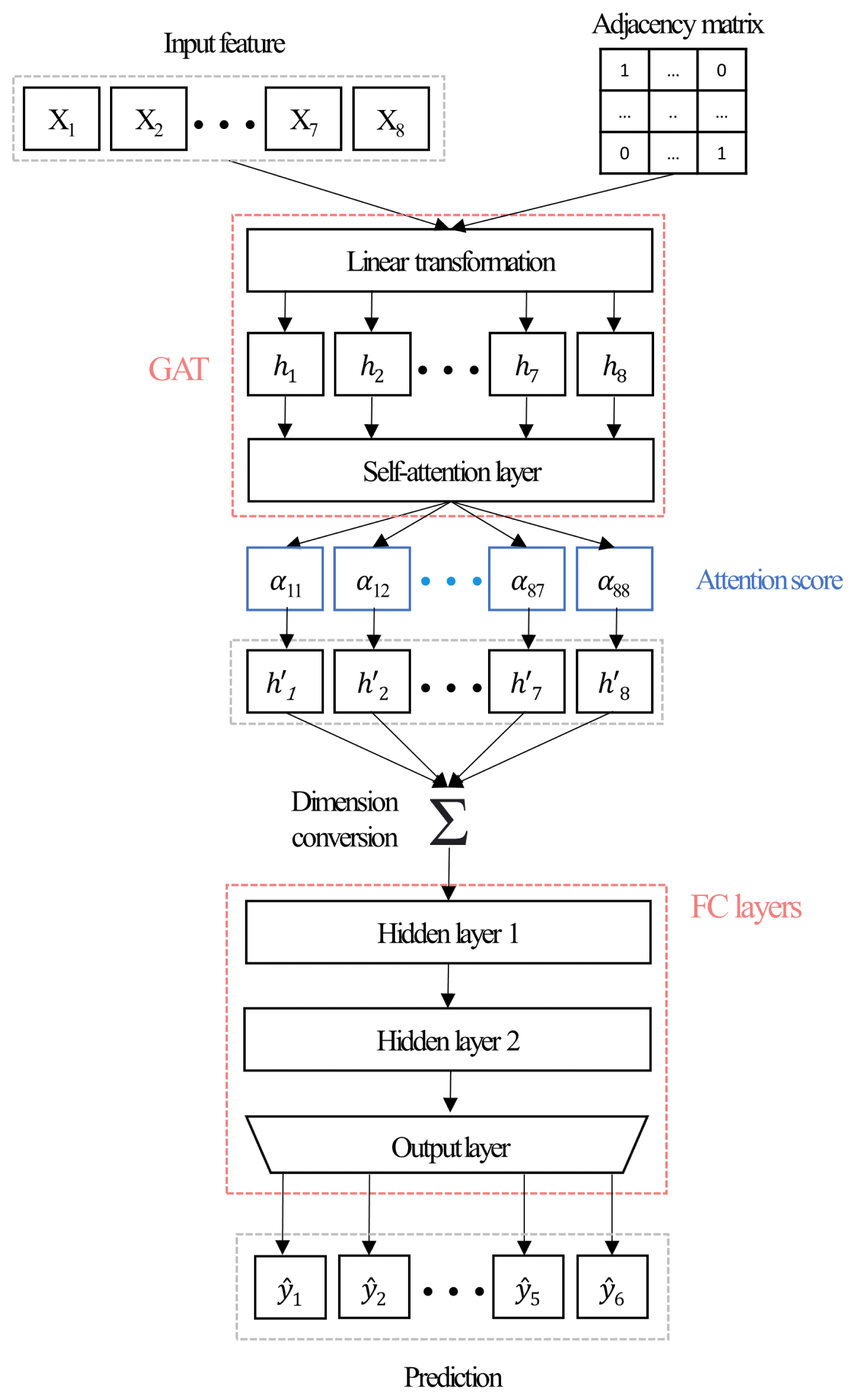

Fig. 3

Schematic of the modeling procedure for forecasting chlorophyll-a. DL: deep learning; DNN_separate: deep neural network for each site; DNN_concat: deep neural network for all sites; GAT DNN: graph attention network combined with DNN_concat.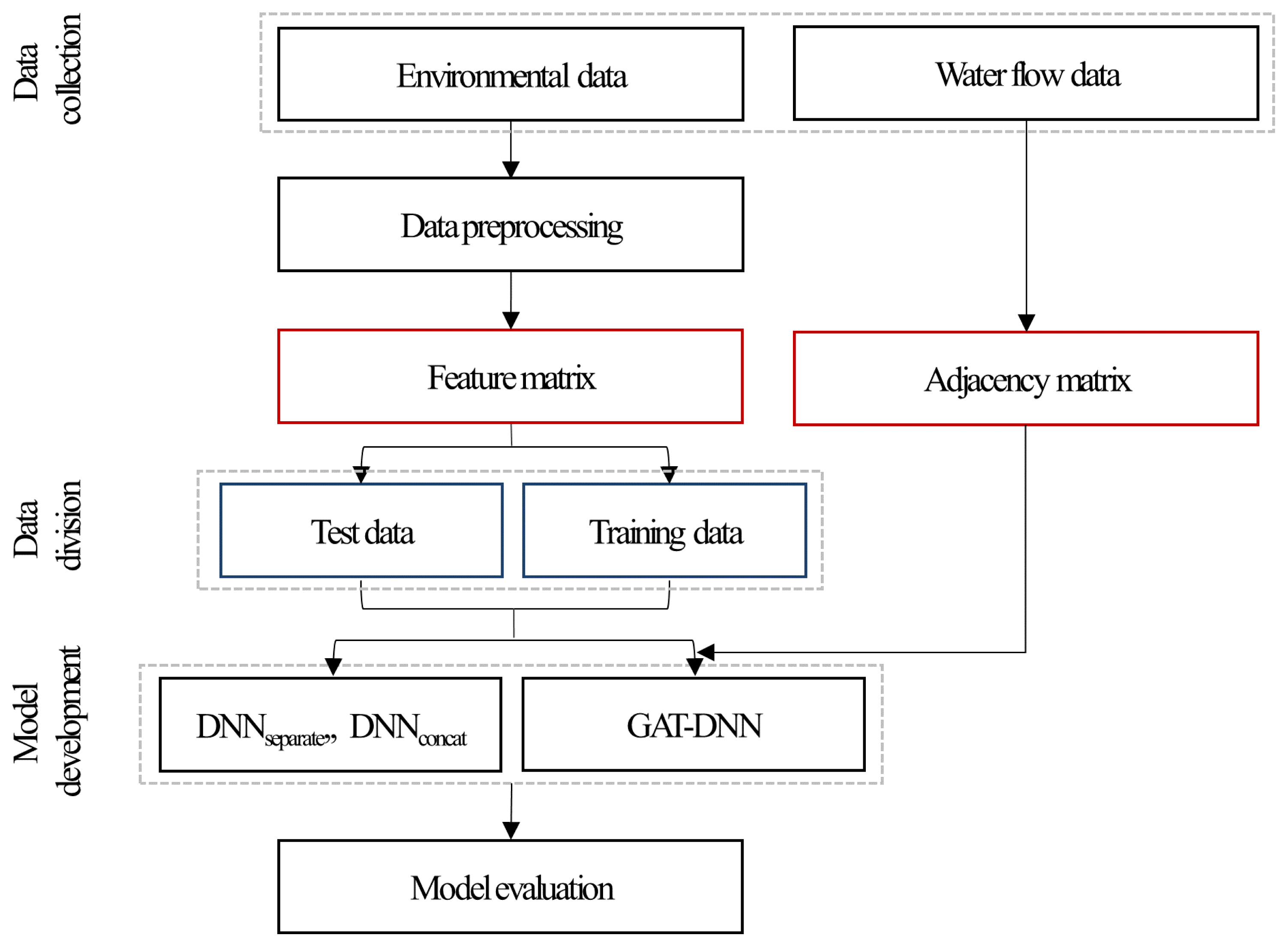

Fig. 4

Chlorophyll-a concentrations at different sites during (a) the summer period (July to September) and (b) other periods from January of 2016 to August of 2022. The log chlorophyll-a concentration of all sites is 1.55 mg/m³ during the summer period (a) and 1.46 mg/m³ during the other periods (b).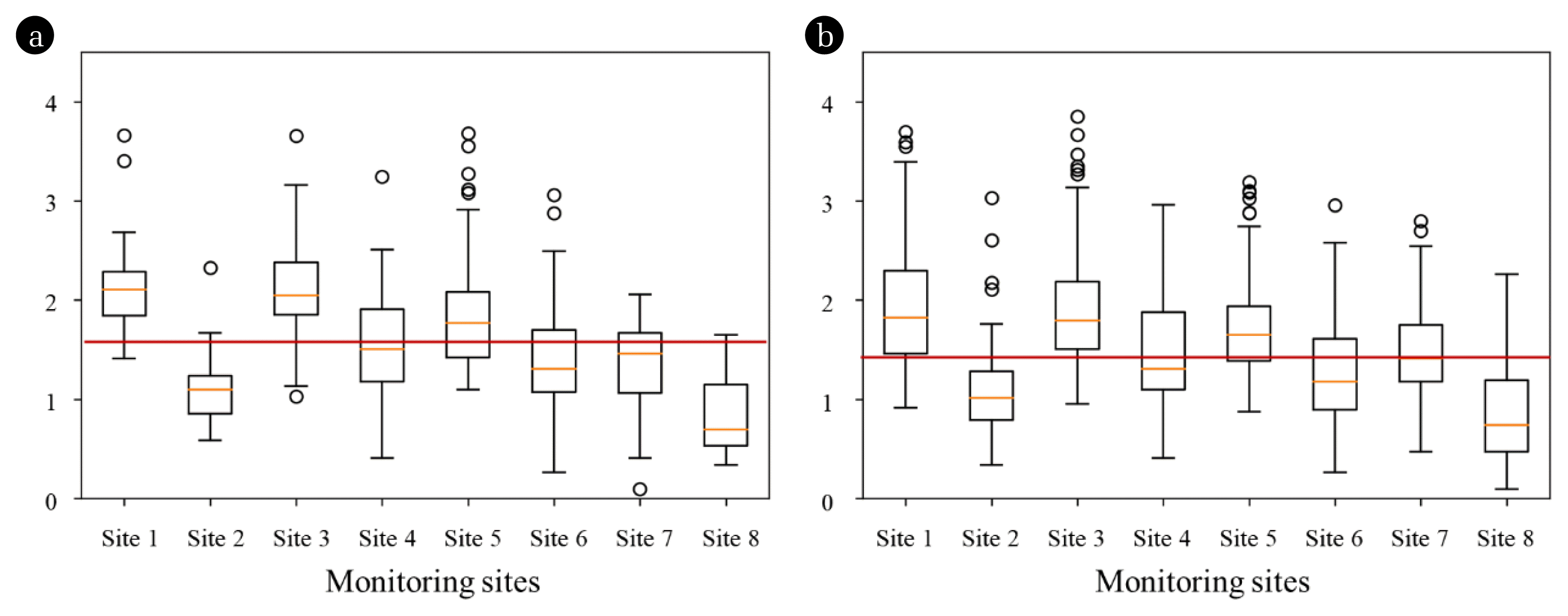

Fig. 5

Comparisons of the measured and GAT DNN-predicted chlorophyll-a concentrations (mg/L) at Sites 1, 2, and 3. In panels (a), (b), and (c), the blue and red circles represent the data in the training and testing sets, respectively. The blue and red lines plot the training and test relationships, respectively, while the black dotted line is the one-to-one line. In panels (d), (e), and (f), the black-bordered circles represent the measured chlorophyll-a concentrations, and the blue and red stars represent the chlorophyll-a concentrations at the training and testing sample sites, respectively.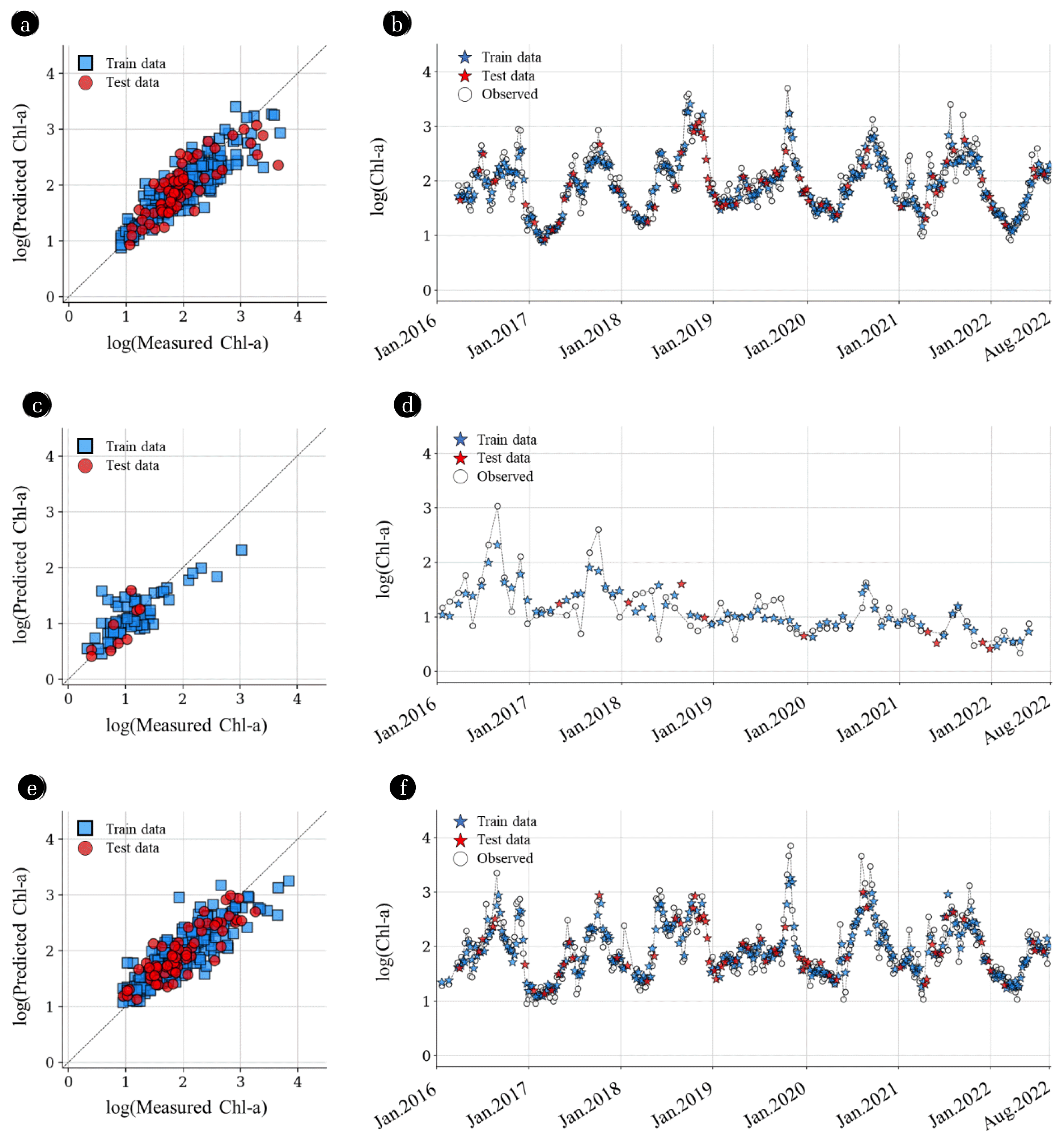

Fig. 6

Similar to Fig. 5, but comparing the measured and GAT DNN-predicted chlorophyll-a concentrations (mg/L) at Sites 4, 5, and 6.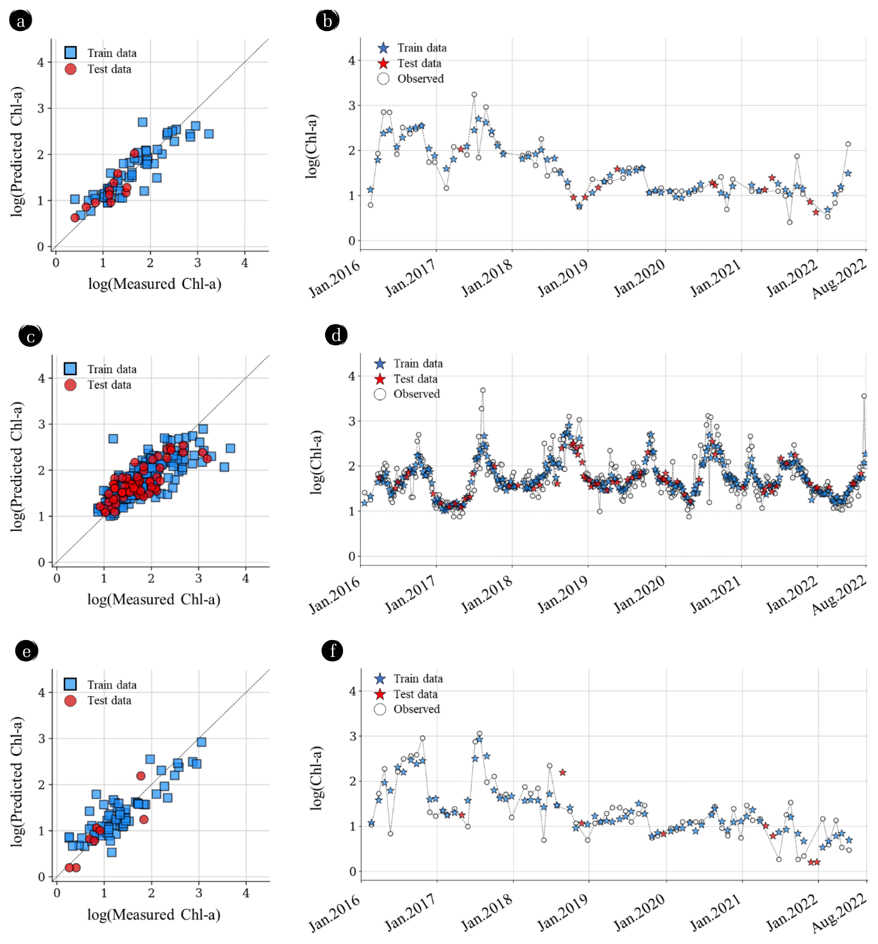

Fig. 7

Test performances of GAT DNN models with different forecast horizons (1 – 6 weeks). Predictions of all sites were made at weekly intervals. Each of six gray lines and associated stars indicates the forecasting performance of GAT DNN for the respective site among Sites 1 and 6, and the black line and associated stars indicates the average forecasting performance of GAT DNN across the sites.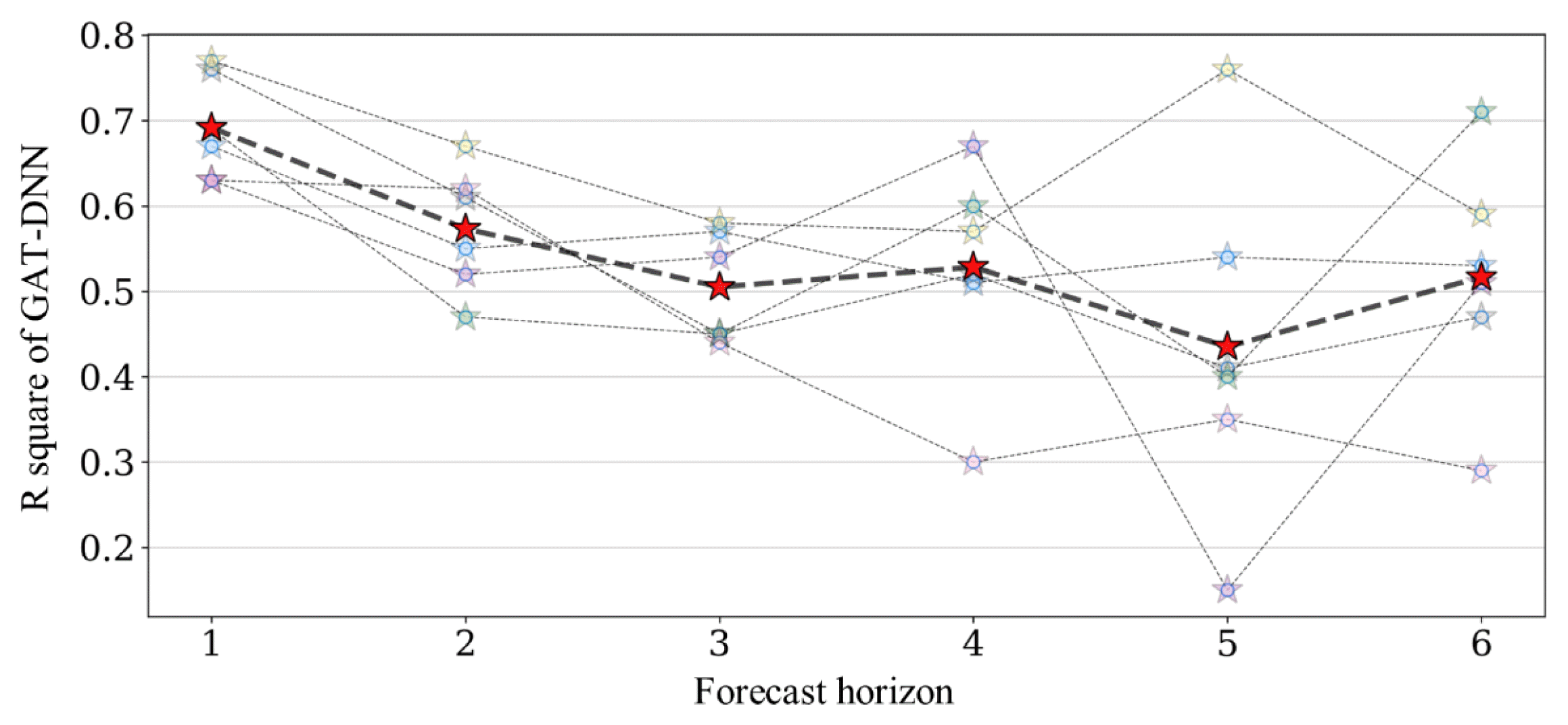

Table 1

Statistical summary of the variables and data sources at Sites 1 – 8. Ranges and means (in parentheses) were calculated based on the measured values in the dataset

Category	Variable	Unit	Site 1	Site 2	Site 3	Site 4	Site 5	Site 6	Site 7	Site 8
Hydrological	Precipitation	mm/day	0–157.5 (4.5)	0–63 (2.5)	0–179 (4.7)	0–68.5 (3.5)	0–179 (4.6)	0–73 (3.3)	0–157.5 (4.0)	0–179 (4.3)
	Total discharge	㎥/s	9.6–789.5 (40.6)	9.6–789.5 (40.6)	9.6–789.5 (40.6)	9.6–789.5 (40.6)	9.6–789.5 (40.6)	9.6–789.5 (40.6)	9.6–789.5 (40.6)	9.6–789.5 (40.6)
Meteorological	Water level	EL.m	67.6–76.9 (72.9)	67.6–76.9 (72.9)	67.6–76.9 (72.9)	67.6–76.9 (72.9)	67.6–76.9 (72.9)	67.6–76.9 (72.9)	67.6–76.9 (72.9)	67.6–76.9 (72.9)
Water quality	TOC	mg/L	1.6–8.1 (2.9)	1.2–3.4 (2.2)	1.2–3.8 (2.3)	1.0–4.0 (2.3)	1.2–3.4 (2.2)	0.9–3.8 (2.3)	1.0–3.8 (2.0)	0.5–5.4 (1.5)
	Water temperature	°C	2.0–32.7 (17.0)	0.5–31.0 (15.3)	0.3–31.0 (15.4)	1.6–31.0 (15.9)	−0.1–31.0 (15.2)	−1.5–31.0 (15.3)	0.5–27.1 (13.7)	0.4–28.6 (13.7)
	DO	mg/L	3.6–10.7 (10.7)	5.6–14.6 (10.1)	6.0–15.9 (10.5)	4.2–18.1 (10.7)	5.5–17.6 (10.5)	3.0–18.3 (10.4)	7.3–16.4 (11.34)	7.2–15.5 (11.02)
	TN	mg/L	0.7–3.3 (1.3)	1.5–3.2 (2.2)	1.4–3.2 (2.1)	1.6–4.4 (2.4)	1.6–4.3 (2.3)	1.5–4.4 (2.3)	0.5–2.7 (1.5)	0.9–5.1 (2.1)
	TP	mg/L	0–0.11 (0.02)	0–0.07 (0.02)	0.01–0.10 (0.02)	0.07–0.12 (0.03)	0.04–0.06 (0.02)	0.05–0.19 (0.02)	0.03–0.13 (0.03)	0.01–0.1 (0.03)
	SS	mg/L	0.2–10.7 (2.3)	0.0–7.6 (1.4)	0.0–9.6 (1.7)	0.4–61.2 (3.0)	0.4–14.0 (1.79)	0.4–67.6 (3.0)	0.3–20.4 (2.8)	0.2–12.5 (2.6)
	Chlorophyll-a	mg/m3	1.5–39.2 (7.4)	0.4–19.7 (2.5)	1.6–45.9 (7.3)	0.5–24.6 (4.6)	1.4–38.7 (5.6)	0.3–20.3 (3.7)	0.1–15.4 (3.8)	0.1–8.6 (1.6)