


1. Introduction
Vegetable fields have been at high risk of heavy metal contamination. Especially with rapid economic development and accelerated urbanization, exploitation and utilization of metals has been increasing. This has resulted in large heavy metals discharges into the soil, posing a serious threat to the quality of farmland and cultivated land [1, 2]. According to the National Soil Pollution Investigation Bulletin [3] issued in April 2014, the total above-standard incidence of soil pollution in China reached 16.1%. At present, the cultivated land polluted by Cd, Pb, Cr and other heavy metals in China is nearly 2×10⁷ ha. In addition, heavy metal levels near factories and mining areas seriously exceed the standard, thus causing regional pollution [4]. For example, studies have shown that the near soil lead-zinc mines was highly polluted [5, 6]. Soil concentrations of many heavy metals such as Pb, Zn and Cd were tens or even hundreds of times higher than the environmental background, posing a serious threat to the growth of local vegetables and the quality of agricultural products [7].
Nanjing is a typical lead-zinc mining area in Eastern China and has been chronically exploited approximately 60 years [8, 9]. During this period, a series of environmental problems have occurred. As a major lead and zinc mining areas, many environmental and soil scientists have researched heavy metals pollution there. Hu et al. [10] evaluated the potential health risks of heavy metals for greenhouse and corresponding open field production by studying soil and vegetable consumption. Chu et al. [11] researched mining, Qixia temple, and vegetable fields, and quantified heavy metal levels in soil with reference to national soil environmental quality standards. Identification of pollutants’ sources is necessary to qualitatively determine the main pollution sources, but also to quantitate the contributions of various sources. Source identification is the top priority for understanding, and key to dealing with, heavy metal pollution. Therefore, it is necessary to strengthen the deep understanding and evaluation of possible ecological risks due to heavy metal pollution. However, studies on the local characteristics and sources of heavy metal pollution have rarely been reported. Soil, as an independent natural body, is time-space continuous and spatially variable [12, 13]. This makes it suitable for application of GIS tools in soil science at both large and small scales [14, 15].
This study aimed to determine the relationships between soil properties (pH, soil organic matter, cation exchange capacity) and the concentrations of heavy metals (Cu, Zn, Cd, As, and Zn) in vegetable soils; to analyze and characterize their spatial distributions; to identify the sources of these heavy metals and evaluate their pollution levels in the complex soil environment; and to provide a scientific basis for the selection of vegetable varieties and rational planning of agricultural production.
2. Materials and Methods
2.1. Study Area
The research area is located northwest of Nanjing, Jiangsu Province (32°02′ 50″ N, 118°45′ 42″ E). The landforms in the territory are intricate, with scattered distribution of low mountains, hills and plains. The terrain fluctuates greatly; altitude ranges from 10 to 300 meters. The annual average temperature is 15.3°C, the frost-free period is 7 months and the annual precipitation in the whole region is about 1,000 mm.
The bedrock consists mainly of gneiss in Nanjing (Fig. S1) and the vegetable fields were reclaimed from landfill on Yangtze River alluvium. The soil type is yellow brown soil [16]. The vegetable fields studied in this experiment are distributed on both sides of a highway. The pH is about 5.0–6.7, and the salt base saturation is 30%–75%. The surface organic matter accumulation is obvious, about 10–20 g/kg. The soil organic matter content decreases with depth, but the clay content increases. Affected by the northern subtropical bioclimatic climate, temperature and rainfall provide favorable conditions for weathering of the parent material, thus forming a viscous core soil layer at depth. It is suitable for planting trees and developing economic forestry, but soil and water conservation are worthy of more attention. Limited by topography, rivers and other factors, the vegetable fields are small and densely distributed. In order to investigate the distributions of soil nutrients and heavy metals, a vegetable field with an area of 0.66 hm2 was selected based on factors such as soil texture, vegetation types and land-use patterns.
2.2. Sample Collection and Analysis
In August 2018, surface (0–20 cm) samples were collected using a grid method with 25 m spacing; each sample was positioned by GPS. The sampling area, about 6,600 m2, was roughly rectangular with a length of 110 meters and a width of 60 meters. A total of 84 points were sampled with a 5 cm diameter soil auger. Three replicates were collected for each point, the soil was mixed and placed in sealed plastic bags and brought back to the laboratory for air-drying.
The soil pH was measured by electrode with a ratio of 1:2.5 between soil and distilled water; soil organic matter (SOM) was determined by wet oxidation at 180°C with a mixture of potassium dichromate and sulfuric acid; cation exchange capacity (CEC) was determined using a 1.0 mol·L−1 ammonium acetate solution. Heavy metals were measured by inductively coupled plasma mass spectrometry (ICP-MS); precision and recovery were tested by spiking reference samples (GSS-1) [17]. By comparison, the recovery of samples was between 86.7–92.6 and satisfied analytical standards.
2.3. Analysis Method
2.3.1. Data statistics
SPSS 22.0 and Excel were used for classical statistical analyses. The Kolmogorov-Smirnov (K-S) test [18] assessed whether data were normally distributed. GS + 9.0 was used to analyze semi-variance and evaluate the spatial continuity of soil variables; Kriging was completed in ArcGIS 9.3 using the parameter model. Correspondence between soil properties and heavy metals was analyzed by correlation analysis, and the source of pollution was analyzed by principal components analysis.
2.3.2. Semi-variance function
Semi-variance function is an important tool in geostatistics to explore soil variability. It can be used to represent the spatial variation structure or spatial continuity of random variables. For random function Z(x) with second order stationarity, the semi-variance (h) can be expressed using the covariance S2 of Z(x) and spatial covariance C(h) as: (h) = S2-C(h), where (h) represents the Z(x) in the spatial relevant, which is equal to mathematical expectation of square of difference value of measured value of interval samples. In general, the semi-variance function increases with the separation distance of samples, finally becoming constant at some distance. The commonly used variation functions include spherical, base station, exponential, and Gaussian models. In this study, according to the multiple fittings of the data, the exponential and spherical models were selected:
Spherical model:
Exponential model:
where h is separation distance, (m); C0 is the nugget value representing the amount of random variation; C1 is the sill, representing structural variance of variable space variation; and A0 is the range, (m). The nugget coefficient is the ratio of the nugget to the sill, which is the value of the function as semi-variance tends to 0, representing random variation caused by measurement errors or variations in soil properties.
2.3.3. The rate of heavy metals exceeding
Referring to soil quality standards, the heavy metal concentration of each sample is compared with the standard values for the first, second and third levels. The exceeding rate for each level is the ratio of the number of samples exceeding the standard to the total number of samples.
2.3.4. The method of Cluster analysis
Cluster analysis [19] refers to a process of grouping a collection of physical or abstract objects into multiple classes composed of similar objects. In essence, the whole process establishes a classification tree. In the establishment process, a threshold can be set on the second part such that when the distance between the last two classes is greater than this threshold, iteration can be terminated. By taking the distance between two samples to get an average value, the overall characteristics of the data are optimized. The shorter the distance between two sets, the greater the similarity. The two most recent classes are then grouped together and the similarity between the newly generated classes and the old classes is recalculated. Iteration continues until all the sample points are in the same category.
2.3.5. Single factor pollution index
The single factor index method refers to evaluation of a single pollutant in the soil. Because it is simple to calculate and can be used to evaluate each pollutant, it has become a relatively common evaluation method at home and abroad [20]. It is calculated as:
where Pi is the pollution index; Ci (mg/kg) is the measured concentration of heavy metal in the soil; and Si is the evaluation standard for that heavy metal. In this experiment, the secondary level standard of soil environmental quality (Table S1) [21] was used as the evaluation standard. If Pi ≤ 1, the sample is not contaminated; samples with Pi > 1 are contaminated, and the greater the value, the more serious the pollution.
2.3.6. The Nemerow integrated pollution index
The Nemerow index method is used to calculate both single-factor and comprehensive pollution indices of soil, and is one of the commonly used methods for comprehensive pollution assessment at home and abroad [22, 23]. The formula can be expressed as:
where P is the comprehensive pollution index of the monitoring points; Pimax is the largest single pollution index; Piavg is the average single pollution index. Soil quality is classified according to P value. The Nemerow comprehensive pollution index was used to determine the pollution level [24]; details are listed in Table S2.
2.3.7. Coefficient of Variation (CV)
The CV is used to compare two groups of data having different measurement scales, or different data dimensions; CV can eliminate the influence of measurement scale and dimension to make an objective comparison. Its calculation formula is [25]:
where SD is the standard deviation, and MN is the mean concentration of soil heavy metal.
3. Results and Discussion
3.1. Descriptive Statistical Analysis
In accordance with national soil nutrient rating standards [26], soil nutrients are rated into six levels, namely, level 1 (very rich, SOM > 40 g/kg, only SOM is described), level 2 (rich, SOM is 30~40 g/kg), level 3 (medium, SOM is 20~30 g/kg), level 4 (deficient, SOM is 10~20 g/kg), level 5 (very deficient, SOM is 6~10 g/kg) and level 6 (extremely deficient, SOM is 0~5 g/kg). As shown in Table S3, soil pH ranged from 4.71 to 7.93; soil organic matter ranged from 13.72 mg/kg to 26.97 mg/kg and CEC from 10.46 mg/kg to 20.47 mg/kg, which were at the deficient and middle levels, respectively. Referring to the secondary evaluation standard of soil environmental quality, except for Cu being within the background range, the levels of Zn, Cd, As and Pb far exceed the background value, reaching 1.85, 5.38, 4.96 and 2.26 times the background value, respectively.
The CV indicates the degree of dispersion between samples and also indirectly reflects the spatial variation of soil indicators. Generally speaking, CV < 0.1 shows weak variation, 0.1 < CV < 1 is moderate variation, and CV > 1 is strong variation. From Table S3, the coefficients of variation of soil pH, SOM, CEC, Cu, Zn, Cd, As and Pb were between 0.08 and 0.34, among which the coefficient of variation of Cu was the lowest (0.08), followed by Pb. Cd had the highest coefficient of variation (0.34), followed by As. Although Pb and Cu showed weak variation, the other indicators showed moderate variation. The CVs of soil indicators followed the descending order: Cd > As> Zn > CEC > SOM > pH > Pb > Cu. Geostatistical analysis requires that data conform to an approximately normal distribution to minimize experimental error [27]. One-sample K-S tests at significance level α = 0.05 showed that the data all conformed to the normal distribution.
The vegetable field selected for this experiment was a typical mining landscape unit with low-lying terrain, densely dissected by rivers and ditches, and greatly disturbed by human activities. Classical statistical analysis showed that the soil pH in the study area was slightly acidic or alkaline, and levels of SOM and CEC were relatively low and moderately variable. One possible reason is that human activities can decrease soil nutrients [28]. In addition, the effects of topography and surface runoff also reduced accumulation of soil nutrients [29].
Some heavy metal standards in these soils were seriously exceeded, although concentrations varied greatly. The most over-standard elements were Cd and As, while Cu was below the nominal pollution threshold. Cu and Pb were slightly variable within the sampling range, and may be regionalized pollutants, which may be related to farmers’ fertilization practices.
3.2. Characteristics of Soil Properties and Semi-Variance Function
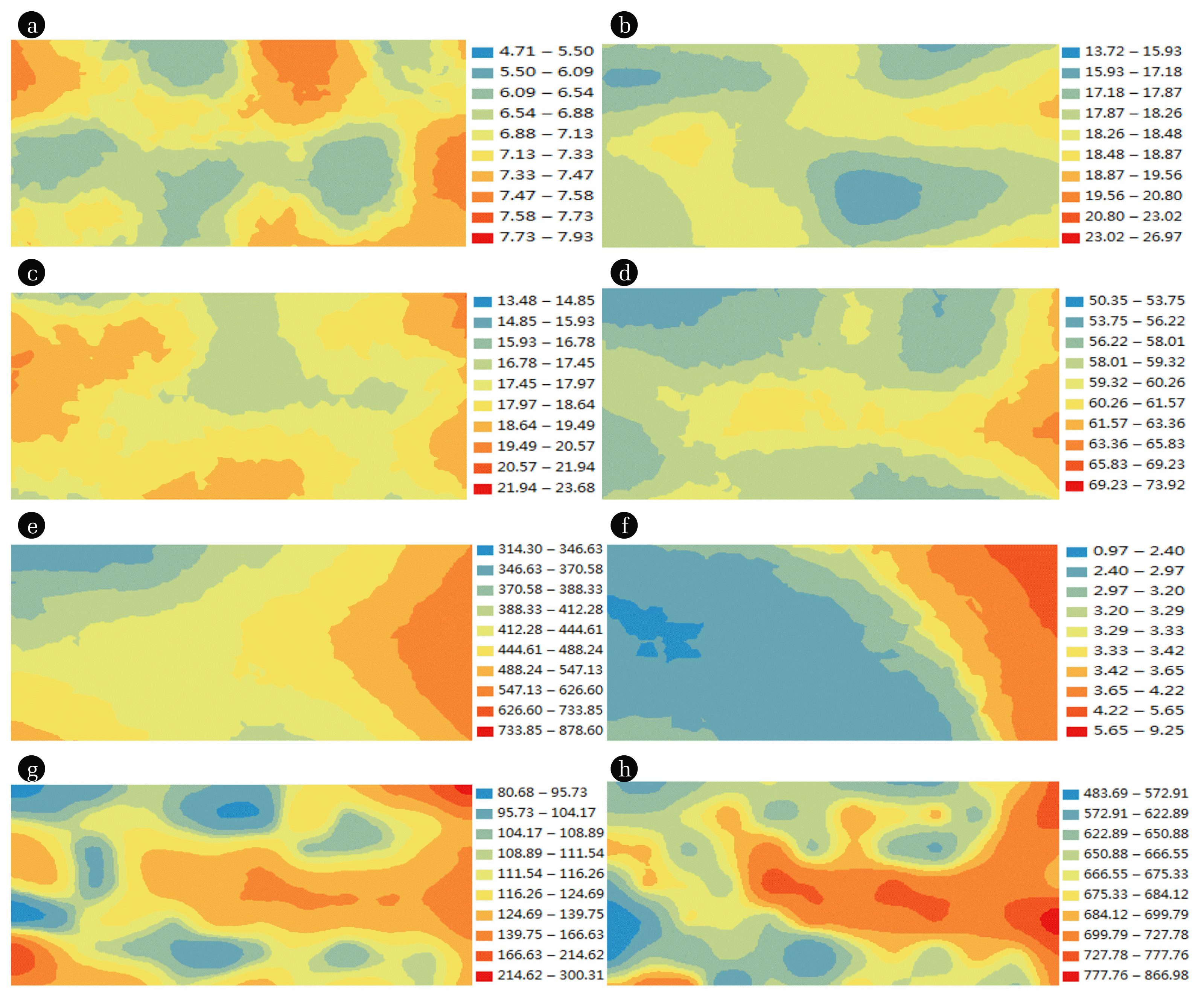
Measured soil parameters were fitted using the geostatistical analysis software GS+ 9.0, and semi-variance functions (Fig. 1) and structural parameters (Table 1) were obtained [30]. The Nugget value (C0) is the corresponding value of the function at the origin, reflecting the random variation within the system; the Sill (C0 + C) represents the total variation within the system; the Range (A0) is the maximum spatial correlation distance, which reflects the physical extent of spatial autocorrelation of the variables. The ratio of Nugget to Sill (C0/C0 + C) is called the Nugget effect, which reflects the spatial dependence of soil properties and indicates the degree of spatial correlation of system variables. When the ratio is less than 25%, the spatial correlation between variables is strong. Between 25% and 75% indicates moderate spatial correlation. When the ratio is more than 75%, the spatial correlation between variables is weak [31, 32].
From Table 1 and Fig. 1, soil indicators in the study area had strong semi-variance structure, and the function well fitted the variation of each index within the sampling range. The results showed As had moderate spatial correlation; the other indicators showed strong spatial correlation. The Nugget of each index followed the descending order: As > Cu > SOM > Cd > pH > Zn > CEC > Pb. Considering range of variation, Zn had the largest range (146.7 m) and better spatial continuity. The correlation range of each indicator was 45.3 ~ 146.7 m, which was larger than the sampling scale (10 m). The results showed that all soil indicators presented evident spatial correlation at the sampling scale of 10 m, and the sampling scale met the requirements of spatial variation analysis. That is, soil properties (pH, SOM, CEC) and five heavy metals (Cu, Zn, Cd, As, Pb) presented their own characteristic distribution in area, direction and shape to some extent by their own value or content.
3.3. Spatial Distribution of Soil Properties and Heavy Metals
As shown in Fig. 2, spatial distributions of soil properties and heavy metals differed in area, direction and shape. pH showed a relatively concentrated patchy distribution, with most values between 6.29 and 7.37. Organic matter showed a scattered patchy distribution, the areas with higher content were distributed around the study area, and the sub-marginal content was generally lower than inside. Generally speaking, the distribution of organic matter was uneven under natural condition. Vegetable farmers in this area spread farm manure along ditches over long periods; this may have caused the scattered patchy SOM distribution. The overall distribution characteristics of CEC were “concave” type (low in the center and higher east and west). It is usually seen that CEC increases with increasing values of pH and SOM. In this study, CEC trends were similar to pH while different from SOM. Therefore, pH and SOM influenced distribution of CEC. Spatial distributions of Cu and Zn were similar, with higher values in the eastern part of the study area, and the lowest contents on both sides. The higher eastern values were due to a copper-zinc deposit nearby. Cu and Zn concentrations were roughly decreased with distance from eastern. The Cd concentration was mostly between 2.40 and 3.29 mg/kg, and gradually increased from the southwest to the northeast. Spatial distributions of As and Pb were similar, but highly fragmented, with no obvious regularity.
3.4. Correlation Analysis
Table 2 shows the correlations between pH, SOM, CEC and the content of heavy metals. Among these, pH and heavy metals were not significantly correlated; soil organic matter was significantly positively correlated with Zn and Cd, and positively correlated with As; CEC was significantly positively correlated with Cu, and positively correlated with Pb. For heavy metals, apart from Cd having no correlation with Zn or Cd, other pairs of elements all had highly significant positive correlation, which proved the complexity of pollution among elements. The results also showed that, within a range, the concentrations and availability of heavy metals decreased with the increase of pH, suggesting that soil pH could be improved by amendments such as lime and biochar [33]. Concentrations of Zn and Cd increased with the increase of organic matter, indicating that the organic matter had a great influence on the bioavailability of heavy metals [34, 35]. In addition, the concentration of Cu increased with the increase of CEC, and decreased with the increase of pH. This phenomenon may be closely related to soil texture and field fertilization.
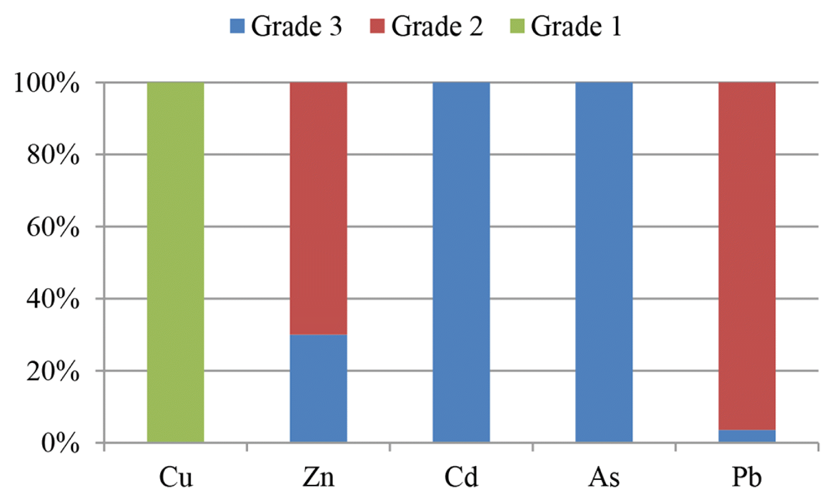
3.5. Standard-Exceeding Concentrations of Elements and Assessment of Heavy Metal Pollution
Referring to national standards [21], the degree of heavy metal pollution is divided into three grades (Table S4). As shown in Fig. 3, the safety of Cu in vegetable soil was 100%, reflecting a nominally low or zero degree of Cu pollution. The other four elements met various levels of pollution. The concentrations of Cd and As at each sampling point exceeded the national third-level standards. On the other hand, the secondary over-standard rate of Zn and Pb reached 70.24% and 96.43%, respectively, indicating that heavy metal pollution in these vegetable plots was prevalent and the data dispersion was small.
As mentioned above, these five elements were taken as pollution evaluation indicators. The degree of heavy metal pollution was evaluated according to the single factor pollution index and the Nemerow comprehensive pollution index (Table 3).
From Table 3, the single factor pollution index of Cu was less than 1, which is a safe level. However, pollution indices of Pb, As, Zn, Cd were greater than 1. The degree of pollution in these vegetable fields was ranked as Cd > As > Pb > Zn. The degree of Cd pollution was the worst, with Nemerow comprehensive index (P) reaching 11.55, while the Nemerow index of As reached 9.19.
The migration rates of heavy metals depend on soil texture; the “stickier” the soil, the slower they move. Soil texture is the consequence of multiple formative factors, including parent material, climate, landform, even biology and development time. Abundant rainfall aggravates soil stickiness in the study area; the more abundant the rainfall, the stickier the soil, resulting in a relatively heavy texture. Heavy metals migrate slowly in this soil and accumulate in the stickier layers. In addition, lead and zinc mining in the nearby Qixia area have also increased the risk of contamination by Cd and As. Based on the results of pollution assessment, it is suggested that in addition to reducing pesticide spraying and fertilizer application, farmers can transfer heavy metals from the soil layer to the ground by plowing. In addition, hyper-accumulative plants such as Viola baoshanica (accumulates Cd) and Centipede (accumulates As) can be planted on vegetable garden soils to absorb and fix heavy metals.
3.6. Principal Component Analysis (PCA)
Table 4 shows the variance contribution rate and cumulative contribution rate of each component. It can be seen that only the eigenvalue of the first principal component was greater than 1 [36, 37]. However, the second principal component eigenvalue was also greater than 1 after rotation of the matrix. Therefore, SPSS extracted the first two principal components, accounting for 83.78% of the total variance, which demonstrated that the extracted two common factors had a strong explanatory power for soil variables.
As shown in Table 4, the first principal component (PC1) explained 46.82% of the total variance and loads heavily on Cu (0.919), Zn (0.770), and Pb (0.868). According to the statistical analysis and local actual situation, Pb and Zn were derived from crustal magmatic rocks and regolith, and gradually formed deposits accumulated on the surface due to continuous excavation and mining, so the presence of these two elements can be attributed to natural sources. Cu mainly came from wastewater discharged from nearby metallurgical plants and introduced into nearby fields through a mixed sewage outlet. Therefore, the PC1 reflected the impact of industrial pollution and mine emissions on vegetable fields.
The contribution rate of the second principal component (PC2) was 36.96%, loading heavily on Cd and As with values 0.918 and 0.828, respectively. Sampling sites in this experiment were in agricultural tillage fields and it can be judged that Cd and As, originating from agricultural pollution, were mainly affected by human activities including fertilizer and pesticide application. On the other hand, Pearson analysis showed a very significant correlation (0.670**) between the two elements, indicating that there may be compound pollution of the two elements. The correlation analysis results further showed the complexity of the pollution of the two elements.
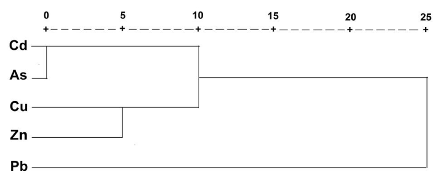
3.7. Cluster Analysis of Five Soil Heavy Metals
As can be seen in Fig. 4, within the range of 10–15, the five heavy metal elements can be roughly divided into three categories: Cd, As and Cu fall into the first category; Cu and Zn fall into the second category; Pb belongs to the third category. Meanwhile, in the first category, Cd and As were more closely related. When the distance was less than 1, Cd and As grouped together, reflecting that the differences between Cd and As in soil were small, and pollution by them may be homologous. At the same time, the average soil concentrations of Cd and As exceeded the secondary evaluation standard for soil environmental quality (GB 15618-1995). The results of cluster analysis were in agreement with those of principal component analysis, providing a basis for further analysis and exploration of the sources of heavy metal pollution.
4. Conclusions
The concentrations and sources of the heavy metals Cu, Zn, Cd, As and Pb in vegetable soil samples were studied. Results showed that this field soil was threatened by four of the heavy metals (excluding Cu); Zn, Cd, As and Pb were contaminants, to varying degrees. Cd and As, the most serious pollutants, were 5.38 and 4.96 times the background values, respectively. Farmers’ fertilization practices played a major role in the variation of soil nutrients in these vegetable fields. Chemical fertilizers (such as phosphates) and pesticides resulted in accumulation of Cd and As.
We tested the correlation between soil properties and heavy metal concentrations and found that the five heavy metals were closely correlated with soil properties. Zn, Cd and As increased with increasing soil organic matter; Cu and Pb increased with soil CEC. However, there was no direct evidence that pH values and heavy metals were correlated. Geostatistical analysis indicated that the soil indicators had measurable spatial variation at the field scale. Multivariate analysis suggested that the heavy metals could be grouped according to their sources: natural and anthropogenic. Pb and Zn mainly originated from a natural source. Cu came from metallurgical waste discharge. As and Pb originated mainly from agricultural pollution.