Numerical study of fluid behavior on protruding shapes within the inlet part of pressurized membrane module using computational fluid dynamics

Changkyoo Choi; Chulmin Lee; No-Suk Park; In S. Kim

doi:10.4491/eer.2018.423

Abstract

This study analyzes the velocity and pressure incurred by protruding shapes installed within the inlet part of a pressurized membrane module during operation to determine the fluid flow distribution. In this paper, to find the flow distribution within a module, it investigates the velocity and pressure values at cross-sectional and outlet planes, and 9 sections classified on outlet plane using computational fluid dynamics. From the Reynolds number (Re), the fluid flow was estimated to be turbulent when the Re exceeded 4,000. In the vertical cross-sectional plane, shape 4 and 6 (round-type protrusion) showed the relatively high velocity of 0.535 m/s and 0.558 m/s, respectively, indicating a uniform flow distribution. From the velocity and pressure at the outlet, shape 4 also displayed a relatively uniform fluid velocity and pressure, indicating that fluid from the inlet rapidly and uniformly reached the outlet, however, from detailed data of velocity, pressure and flowrate obtained from 9 sections at the outlet, shape 6 revealed the low standard deviations for each section. Therefore, shape 6 was deemed to induce the ideal flow, since it maintained a uniform pressure, velocity and flowrate distribution.

Keywords: Computational fluid dynamics, Fluid pressure, Fluid velocity, Pressurized membrane module design, Protruding shapes

1. Introduction

Microfiltration (MF) and ultrafiltration (UF) have been used in pressurized membrane modules that can be applied across multiple fields, including chemical, food, pharmaceutical, and water treatment industries. Important UF membrane designs employ a hollow fiber configuration, as advantages of this membrane are its low cost and high surface area unit per volume. Subsequent applications have confirmed that the pressurized modules of UF hollow fiber membrane are economically attractive and effective [1, 2].

The performance of most pressurized membrane modules, however, is limited by the concentration polarization and membrane fouling, which hinder module productivity due to the flux decrease [3]. Pressure-based membrane processes have played key roles in industrial operations due to their operating conditions and cost effectiveness [4, 5].

To improve the performance of pressurized membrane modules, fluid distribution, e.g., velocity, pressure, and streamline within the module, is an important factor for indirectly evaluating the flux. In addition, variations of the velocity, pressure, and streamline can be used to estimate local membrane fouling, as the fluid flow concentrates in parts of the membrane module. However, considerable experimental time and manufacturing costs are wasted when a real module is used to evaluate the flux in module configurations. To overcome these difficulties, computational fluid dynamics (CFD) have been often used.

CFD has recently become a tool available for analyzing membrane filtration systems, due to the rapid development of computational performance and mathematical methods [6]. Changes in the pressurized membrane module affect fluid distribution, and increased the flux in the membrane module [7]. In general, CFD methods have proposed the use of numerical methods using a computer in order to analyze the fluid flow. The basic principle of CFD is to use discretized algebraic equations approximated from the partial differential equations of viscous fluid flow [8].

A large number of studies have been performed over the last two decades, which investigate the effects of different types of baffles, spacers, and other turbulent promoters, in addition to their orientation and spatial configuration, on flow hydrodynamics and concentration boundary layer disruption [9–12].

In other studies, Zhuang et al. [13] investigated the impact of the shell manifold on the performance of a hollow-fiber membrane module using dead-end outside-in filtration. From these results, the CFD model was found to be beneficial in interpreting the structure design and optimization of the hollow-fiber membrane modules. Liang et al. [14] analyzed the effect of membrane properties and bulk flow conditions to identify whether electro-osmosis alone was effective for improving the mass transfer and permeate flux in a steady-state. As a results, it was confirmed that electro-osmosis led to a permeate flux increase of 0.5% to 11%. Liu et al. [3] investigated the effect of each type of baffle, e.g., central baffles or wall baffles in membrane tubes, on the flow pattern and behavior. They revealed that both types tend to reduce the concentration polarization and membrane fouling. Ghidossi et al. [2] defined the flow mechanism in the module and calculated the pressure drop for all UF system configurations using FLUENT. Based on their work, the pressure drop was found to be greater at a higher inlet pressure and lower when the permeability increased; the pressure drop was quasi-linear along the entire membrane length. Vinther et al. [15] presented the effect of back-shocking in UF using two dimensional mathematical models. As a result, it revealed that the optimal back-shock time from CFD was in good agreement with the data from literature.

From a literature review, it has been found that CFD can be used to estimate the fluid flow-through velocity and pressure values at the inlet and outlet, and as such can also be used to calculate the permeability for membrane module configurations. This paper further analyzes the effect of fluid flow for protruding shapes at the inflow to determine which protruding shape induces a better flow pattern when the module operates, by investigating the velocity and pressure in the entire module, using a vertical cross-section of the module, outlet, and nine sections of the outlet plane.

2. Simulation Set-up

2.1. Governing Equations

Fluid behavior is often counterintuitive, making it difficult, if not impossible, to predict the impact of fluid flow. CFD is a tool that has successfully been used to simulate the behavior of fluid flow (www.ansys.com). Some of commonly used CFD software includes: FLUENT, CFX, FLOWIZARD, PHOENICS, STAR-CD, and OPEN FOAM [16].

In this study, to simulate the internal fluid movement, ANSYS CFX (version 18.0) was employed. CFX is a high-performance CFD software tool that has displayed outstanding accuracy in its hydraulic analysis of membrane modules [17]. At the heart of CFX is its advanced solver technology, the key to quickly and robustly achieving reliable and accurate solutions.

The governing equation of ANSYS CFX is the Navier-Stokes equation, which describes conservation and transport processes. This fluid is assumed to be Newtonian when the flow is in a steady state and laminar Eq. (1) [18].

(1)

\frac{\partial u}{\partial x} + \frac{\partial v}{\partial y} + \frac{\partial w}{\partial z} = 0

where u is the velocity in x direction, v is the velocity in y direction, and w is the velocity in z direction.

K-epsilon (k-ɛ) model is commonly employed to interpret flow properties for turbulence conditions in CFD [19]. There are two variables of turbulence kinetic energy (k) and the rate of dissipation of turbulence energy (ɛ) in this model. The turbulent viscosity is assumed as isotropy that the ratio between Reynolds stress and deformation rate is the same in all directions [20]. The k-ɛ equations have a lot of unknown terms. To practically approach, the standard k-ɛ model is employed to minimize the unknown factors, thus applying a plenty of turbulent flow applications. The equations of turbulent kinetic energy (k) and dissipation (ɛ) are follows [21].

(2)

k : \frac{\partial (ρ k)}{\partial t} + \frac{\partial (ρ k u_{i})}{\partial x_{i}} = \frac{\partial}{\partial x_{j}} [\frac{μ t}{σ_{k}} \frac{\partial k}{\partial x_{j}}] + 2 μ_{t} E_{i j} E_{i j} - ρ ɛ

(3)

ɛ : \frac{\partial (ρ ɛ)}{\partial t} + \frac{\partial (ρ ɛ u_{i})}{\partial x_{i}} = \frac{\partial}{\partial x_{j}} [\frac{μ t}{σ_{ɛ}} \frac{\partial ɛ}{\partial x_{j}}] + C_{1 ɛ} 2 μ_{t} E_{i j} E_{i j} - C_{2 ɛ} ρ \frac{ɛ^{2}}{k}

where u_i is velocity component in corresponding direction, E_ij is component of deformation rate, and μ_t is eddy viscosity.

2.2. Module Structure

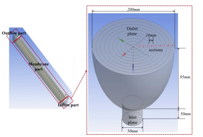
The pressurized membrane module consists of inflow, membrane, and outflow parts. In this study, the CFD simulation was performed at the inflow of the module. The inflow part is a down-to-up flow, the lower section is the inlet, and the upper is the outlet, as shown in Fig. 1. The center part (bottom of core tube with 40 mm diameter) of the outlet plane does not permit flow due to the core tube in the membrane for the permeate. Overall, the outlet plane was comprised of nine sections, except for the center hole.

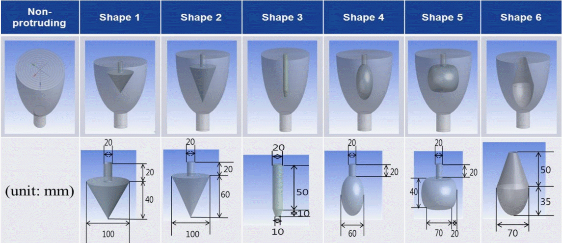
The shape of the protruding part is as follows: shape 1 is a small triangle, shape 2 is a large triangle, and shape 3 is a long bar, shape 4 is a circle, shape 5 is an ellipse, and shape 6 is a modified round shape. The protruding part considered in this paper is finally determined as 6 shapes excluded the angular shape in order to smooth fluid flow. The detailed specifications of the protruding shapes are shown in Fig. 2.

2.3. Boundary Conditions

Simulations in this study were conducted using 3D flows. In the CFD, the boundary condition can be set based on the flowrate, pressure, and velocity. Since the velocity and the pressure values at the inlet and outlet are not consistent and are obtained as the results, the boundary condition is set as the flowrate in this study.

The flowrate at the inlet was 1.9625 L/s at a velocity of 1 m/s and a diameter of 50 mm. The flowrate at the outlet was set at 0.3925 L/s, assuming that every flowrate of the inlet passes through the outlet. The total effective area at the outlet per total effective area at the inlet was 1/5 at 6,358.5 m²/31,400 m² when 10,000 fibers (generally 9,000–10,000 fibers per module) were employed in the membrane. The detailed conditions of the inflow are shown in Table 1. The wall boundary conditions were applied under non-slip conditions.

2.4. Reynolds Number

In this study, the Reynolds number (Re) was analyzed prior to each simulation to determine the dominant flow in this module (e.g., laminar or turbulent). The Re is an important dimensionless quantity in fluid mechanics used to help predict flow patterns in different fluid flow situations, and also to estimate the transition from laminar to turbulent flow. Laminar flow implies a low Re, where viscous forces are dominant, and is characterized by a smooth and constant flow motion (Re < 2,300). A turbulent flow implies a high Re, dominated by inertial forces, which tend to produce chaotic eddies, vortices, and other flow instabilities (Re > 4,000). Transient flow has the Re range between 2,300 and 4,000.

The Re represents different flowrates through the systems based on the following equation [22]:

(4)

R e = \frac{ρ u D}{μ}

where u is the average velocity (m/s) on vessel, D is the vessel diameter (m), ρ is the water density (kg/m³), and μ is the dynamic viscosity (Pa•S) of water.

Here, the Re was derived from four points, e.g., the inlet, 50 mm and 90 mm from the inlet, and the outlet, in order to determine the Re at the inflow. The locations of the four points measured are shown in Fig. S1.

3. Results and Discussion

3.1. Hydraulic Re

The Re is affected by the effective area, effect volume, and velocity on the protruding shape in the inflow. As described above, the Re is derived from measurement taken at the inlet, 50 mm and 90 mm from inlet, and the outlet, under laminar and turbulent flow conditions in order to confirm whether the fluid flow in the inflow is laminar or turbulent; the calculated Re values from the CFD simulations are shown in Table S1.

Analytical results of the CFD showed that the Re was turbulent at much higher than 4,000 under all conditions (e.g., no protruding, and shapes 1 to 6). Also, the Re values at the inlet, 90 mm from the inlet, and the outlet were considerably larger than at inlet and 50 mm from inlet because the effective area of the outlet was 1/5 smaller than the inlet effective area. This difference is because the upstream flow and the downstream flow collide at 50 mm from inlet, where the reverse flow phenomenon occurs and the velocity sharply decreases. In addition, the Re of shapes 5 and 6 were relatively lower at the outlet compared to the other shapes, suggesting that the fluid flow changed due to the protruding shape.

From the above results, the Re of fluid flow in the inflow part was found to be strongly turbulent at over 4,000. Hence, turbulent mode was deemed appropriate for simulating the CFD of the velocity and pressure in the inflow.

3.2. Variations of Velocity and Pressure at Cross-sectional Plane

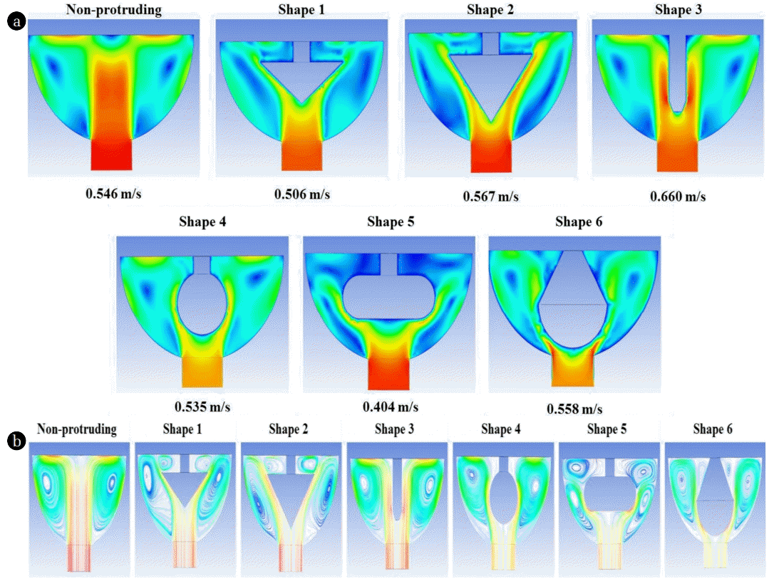
3.2.1. Cross-sectional plane contour, average, and streamline velocity

In turbulent flow mode, the CFD simulation of the inflow reveals the flow velocity profile in the vertical cross-section (Fig. 3). The intensity of velocity in the contour can be interpreted as follows: red > orange > yellow > green > sky blue > blue. The large amount of red and blue in the inflow implies that the fluid flow is localized, whereas abundant orange, yellow, green, and sky blue implies that that the flow is relatively evenly distributed.

From the contours and average velocity values of the vertical cross-sectional plane, primarily red was seen at the no protruding, and shapes 1, 2, 3, 5; among these, shapes 1, 2, and 5 showed some blue color, especially at the bottom part of the protrusion, indicating severe localization of the fluid flow. In contrast, shapes 4 and 6 showed a relatively uniform flow distribution, with primarily orange, yellow, green, and sky blue in the inflow.

In the cross-sectional plane of the velocity streamline, plenty of fluid flowed from the inlet to outlet at the center in the no protruding and shape 3, with large vortices occurring on both sides of the inflow. Shapes 1, 2, and 5 displayed a large surface area at the bottom of the protrusions and had small vortices, as the fluid could not flow smoothly into the inflow. Due to the protruding shape, shape 6 has a dead space with little fluid flow at the bottom center of the protrusion. The fluid in shape 4 appeared to be evenly distributed within the inflow part because the fluid velocity from the inlet was not seen to be biased to the center, and the vortexes were small. In addition, Liu et al. [3] reported that water flow stagnates and particles tend to accumulate when central baffles are installed in waterways, hence it is expected that water passage will be degraded due to the accumulation of particles when the bottom area of a protruding part is relatively large as shapes 1, 2, and 5 [3].

The average velocity at the cross-sectional plane was 0.535 m/s at shape 4 and 0.558 m/s at shape 6, which are mostly orange, yellow and green colors in the inlet part. From these results, the fluid flow velocity was most uniform for shapes 4 and 6, which are round shapes, rather than triangle, bar, and oval used in shapes 1, 2, 3, and 5.

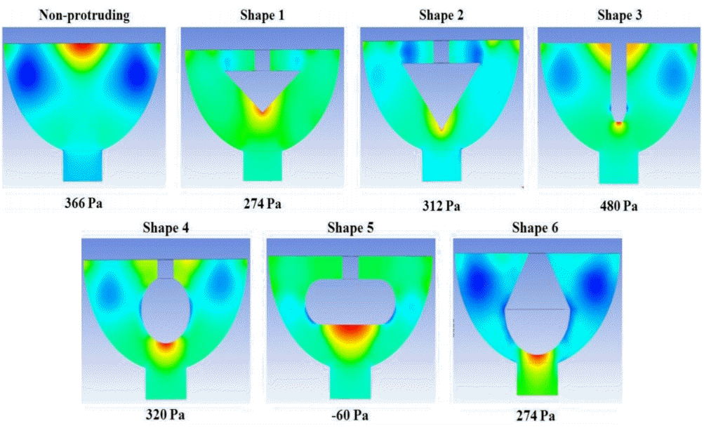
3.2.2. Cross-sectional plane contour and average pressure

The vertical cross-sectional plane of the pressure contour and average at the inflow part under turbulent mode is shown in Fig. 4. As for the velocity, the intensity of pressure in the contour can be interpreted as follows: red > orange > yellow > green > sky blue > blue, with red, orange, and yellow indicating that the fluid flow is stagnant at that point and that the water pressure is high. Green, sky blue, and blue indicate that the fluid passes rapidly at that point, and that the water pressure is low.

From the vertical cross-sectional plane, the contour of the fluid flow is seen to be stagnated at the outlet center of the no protruding and the upper center of the protrusion in shape 5. In contrast, the water pressure was low on both sides at the center of the inflow part, with plenty of water flowing at that point. In the case of shape 2, the protrusion induced a blue color at the bottom, indicating that water flowing into the bottom circulated at that point due to the larger triangle than in shape 1. Shape 6 showed that the water is stagnant at high pressure in the upper part of the protrusion; the fluid flowing out to the outlet circulated on both sides and the water pressure was low. However, in the case of shapes 1 and 4, the pressure distribution was relatively uniform; indicating that the fluid flow was well distributed throughout the inflow.

In the vertical cross-sectional plane, the average pressure values of shape 1 and 6 displayed the low water pressure at 274 Pa, indicating that the water pressure was evenly maintained in the inlet part. In shape 5, the average water pressure was negative (−60 Pa), due to the fact that the fluid flow did not move smoothly at the upper and bottom parts of the protrusions, resulting in a dead space at that point. Note that the results for the water pressure are similar to those for the velocity.

In Fig. 4, the low water pressure distribution was measured in shape 6, which also displayed the high velocity (Fig. 3). Therefore, shape 6 was deemed to permit the best fluid flow.

3.3. Variations of Velocity and Pressure at Outlet

The contour and average velocity at the outlet under turbulent mode are shown in Fig. S2. In terms of contour and velocity, the velocity of the no protruding and shape 3 was concentrated in areas excluding the center and edge. In addition, there was a low velocity at the center of shape 5 and the edges of shapes 2 and 6. In contrast, shapes 4 and 6 showed a relatively high and uniform velocity distribution throughout the outlet.

In the results of the average velocity at the outlet, the shape 3 and 4 were high at 0.853 m/s and 0.736 m/s, respectively. In the case of the no protruding and shape 3, the high flowrate was concentrated at the central part of the outlet due to the high velocity at that point. In contrast, shape 4 displayed both a high velocity and uniform fluid flow.

In terms of the contour and average velocity at the outlet, shape 4 displayed the high velocity and most uniform flow pattern due to the protruding round shape.

The results of the contour and average pressure at the outlet under turbulent mode are shown in Fig. S3. In the case of the contour at the outlet plane, the no protruding and shape 3 primarily displayed red and orange colors at the center of the outlet, indicating that most fluid flowed at that point. The no protruding and shapes 2 and 6 displayed some dead space (blue), indicating that a localization of the fluid flow occurred. Shapes 1, 4, and 5 presented a relatively constant water pressure distribution throughout the outlet.

From the average pressure at the outlet, the no protruding and shapes 3 and 4 had the highest water pressure (445 Pa, 704 Pa, and 470 Pa, respectively), with shape 4 displaying a relatively uniform water pressure at the outlet. Interestingly, shape 5 revealed a negative pressure, as a stagnant space occurred at the center of the outlet.

Therefore, from the results of the contour and average pressure at the outlet, the best conditions for fluid flow were found in shape 4, in terms of hydraulic pressure distribution.

3.4. Flow Distribution on Outlet

3.4.1. Velocity variation at each section on outlet

Fig. 5 presents the velocities and standard deviations for each section with 10 mm interval of the outlet plane. The velocities of shape 3 and 4 at the outlet were high in sections 3, 4, 5, 6 and 7, and low in sections 1, 2 and 9, No protruding condition showed the same tendency as for the shape 3 and 4. Shape 1 and 2 showed that sections 3 and 4 were the highest and section 6 was the lowest. Shapes 5 and 6 displayed the smallest velocity differences for each section, and maintained a low velocity overall.

The standard deviation for the protruding shapes at the outlet was larger when the average velocity was higher and smaller when it was lower. The no protruding and shape 3 had a high mean velocities of 0.647 m/s and 0.837 m/s, respectively, and standard deviations of 0.243 m/s and 0.837 m/s, as the fluid flow was severely concentrated in sections 3 to 7 due to the absence of protrusions or by small interferences in the fluid flow from the inlet by the bar shape. Compared to the no protruding and shape 3, the standard deviations for every section of the outlet in shape 4 were relatively lower at 0.162 m/s, even though the average velocity was high at 0.162 m/s. Shape 5 had the lowest standard deviation at 0.039 for each section, but also had the lowest average velocity of 0.252 m/s. In shape 6, the standard deviation was 0.061 m/s, then average velocity was 0.413 m/s. From these results, the shape 6 has shown the best uniform distribution in the outlet plane, showing a lower standard deviation but a high velocity of 60% larger than shape 5, due the fact that the fluid flow from inlet to outlet was highly interfered by its protrusion.

3.4.2. Pressure variation at each section on outlet

Fig. 6 shows the pressure values and standard deviations for each section of the outlet. The pressure at the outlet for the no protruding and shape 3 was high in sections 1, 2, and 3 and low in sections 5, 6, and 7, indicating that the fluid flow was biased. Shapes 1 and 2 displayed a high water pressure in sections 5, 6, and 7, and low pressure in sections 2, 3, 4, and 8, indicating that they were affected by the protruding shapes. In contrast, shapes 5 and 6 maintained a relatively constant pressure variation for every section of the outlet.

In terms of standard deviation and mean pressure for the protruding shapes, the no protruding and shape 3 had the largest standard deviation of 172 Pa and 174 Pa, respectively. Conversely, shape 4 had a large standard deviation of 134 Pa for each section, with the largest mean pressure of 284 Pa, indicating a well distributed fluid flow at the outlet. Shape 5 had the smallest standard deviation of 19 Pa, but a negative pressure was maintained at an average pressure of −149 Pa. Shape 6 had a low standard deviation of 46 Pa, and the average pressure was low at 41 Pa, indicating that the fluid flowed poorly from the inlet to the outlet.

3.4.3. Flowrate at each section on outlet

As shown in Table 2, the water in non-protruding flowed in sections 1 to 7 of the outlet plane; on the other hand, it was not passed in sections 8 and 9. In shape 1 to 4, there was almost no water flow in the center part (sections 1 to 6) of the outlet plane, while all water flow was concentrated among sections 7 to 9. Shape 5 and 6 exhibited the highest flow rate in section 9, although water was not biased at the center and edge part compared to other shapes.

From the standard deviation of flowrate on sections, non-protruding showed the lowest value, however, no water was passed in section 8 and 9, and it presented that flow tends to be biased on outlet plane. On the contrary, shape 6 showed that water flowed in all sections while maintaining a low standard deviation, indicating that the water distribution was well achieved.

In conclusion, as Monfared et al. [23] reported that the large fluid velocity is high turbulent kinetic energy and that this configuration can have large flowrate, the shape 6 with the highest average fluid velocity in the module has the largest flowrate.

4. Conclusions

The intent of this study was to investigate the effect on fluid flow of protruding shapes installed within the inlet part of pressurized membrane module. The results are as follows.

In the results of Re used to determine the flow pattern of the inflow, Re values were estimated to be under turbulent flow for Re ≫ 4,000, as a whole.
In the contour, average velocity, and pressure in the cross-sectional plane of the inflow obtained using CFD simulations, the fluid velocity of shapes 4 and 6, round-type protrusion, displayed a more uniform flow distribution than other shapes (e.g., triangle, bar, and ellipse), and the fluid pressure in shape 6 maintained the low water pressure. Overall, shape 6 displayed the best fluid flow in terms of velocity and pressure.
From the contour at outlet plane, average velocity, and pressure at the outlet, shapes 4 and 6 with round-type protrusions presented a relatively uniform fluid velocity, and the fluid pressure in shape 4 was found to have better water pressure.
In the simulations of velocity, pressure and flowrate of nine sections at 10 mm intervals on the outlet, the shape 6 was considered to be the best uniform distribution in the outlet plane, showing a high velocity and a lower standard deviation of flowrate on each section.
In summary, shape 6 showed higher average velocity on the cross-sectional and outlet plane of the module, and the standard deviation of flowrate on each section of outlet plane is lowest. Therefore, it proved that shape 6 has the most uniform flow distribution within the module.

References

1. Veríssimo S, Peinemann KV, Bordado J. New composite hollow fiber membrane for nanofiltration. Desalination. 2005;184:1–11.
2. Ghidossi R, Daurelle JV, Veyret D, Moulin P. Simplified CFD approach of a hollow fiber ultrafiltration system. Chem Eng J. 2006;123:117–125.
3. Liu Y, He G, Liu X, Xiao G, Li B. CFD simulations of turbulent flow in baffle-filled membrane tubes. Sep Purif Technol. 2009;67:14–20.
4. Ghidossi R, Veyret D, Moulin P. Computational fluid dynamics applied to membranes: state of the art and opportunities. Chem Eng Proc. 2006;45:437–454.
5. Zare M, Ashtiani FZ, Fouladitajar A. CFD modeling and simulation of concentration polarization in microfiltration of oil-water emulsions; Application of an Eulerian multiphase model. Desalination. 2013;324:37–47.
6. Keir G, Jegatheesan V. A review of computational fluid dynamics applications in pressure-driven membrane filtration. Rev Environ Sci Biotechnol. 2014;13:183–201.
7. Vinther F, Jonsson AS. Modelling of optimal back-shock frequency in hollow fibre ultrafiltration membranes I: Computational fluid dynamics. J Membr Sci. 2016;506:130–136.
8. Munson BR, Young DF, Okiishi TH. Fundamentals of fluid mechanics. 4th ed.New York: Wiley; 2002.
9. Santos JLC, Geraldes V, Velizarov S, Crespo JG. Investigation of flow patterns and mass transfer in membrane module channels filled with flow-aligned spacers using computational fluid dynamics (CFD). J Membr Sci. 2007;305:103–117.
10. Ahmed S, Seraji MT, Jahedi J, Hashib MA. Application of CFD for simulation of a baffled tubular membrane. Chem Eng Res Des. 2012;90:600–608.
11. Shakaib M, Hasani SMF, Mahmood M. CFD modeling for flow and mass transfer in spacer-obstructed membrane feed channels. J Membr Sci. 2009;326:270–284.
12. Ahmed S, Seraji MT, Jahedi J, Hashib MA. CFD simulation of turbulence promoters in a tubular membrane channel. Desalination. 2011;276:191–198.
13. Zhuang L, Guo H, Dai G, Xu Z. Effect of the inlet manifold on the performance of a hollow fiber membrane module-A CFD study. J Membr Sci. 2017;526:73–93.
14. Liang YY, Chapman MB, Fimbres-Weihs GA, Wiley DE. CFD modelling of electro-osmotic permeate flux enhancement on the feed side of a membrane module. J Membr Sci. 2014;470:378–388.
15. Vinther F, Pinelo M, Brons M, Jonsson G, Meyer AS. Predicting optimal back-shock times in ultrafiltration hollow fiber modules II: Effect of inlet flow and concentration dependent viscosity. J Membr Sci. 2015;493:486–495.
16. Sharma C, Malhotra D, Rathore AS. Review of computational fluid dynamics applications in biotechnology processes. Biotechnol Prog. 2011;27:1497–1510.
17. Oh JI, Choi JW, Lim JL, Kim DI, Park NS. A study on hydraulic modifications of low-pressure membrane inlet structure with CFD and PIV techniques. J Korean Soc Environ Eng. 2015;37:607–618.
18. Kavianipour O, Ingram GD, Vuthaluru HB. Investigation into the effectiveness of feed spacer configurations for reverse osmosis membrane modules using Computational Fluid Dynamics. J Membr Sci. 2017;526:156–171.
20. Versteeg HK, Malalasekera W. An introduction to computational fluid dynamics: The finite volume Method. United Kingdom: Pearson Education Limited; 2007.
21. Launder BE, Spalding DB. The numerical computation of turbulent flows. Comput Method Appl Mech Eng. 1974;3:269–289.
22. Taesung S&E Korea. CFX manual: Lecture 10 Turbulence: Introduction to ANSYS CFX. Anflux; [cited 07 November 2017]. Available from: https://www.tsne.co.kr/
23. Monfared MA, Kasiri N, Salahi A, Mohammadi T. CFD simulation of baffles arrangement for gelatin-water ultrafiltration in rectangular channel. Desalination. 2012;284:288–296.
Fig. 1
Structure and specifications of the inflow part.
Fig. 2
Detailed specifications of the protruding shapes.
Fig. 3
Cross-sectional planes of the contour, average, and streamline velocity images: (a) Contour and average velocity, and (b) Velocity streamline.
Fig. 4
Cross-sectional plane of contours and average pressure.
Fig. 5
Velocity variations for sections at the outlet: (a) Velocities and (b) Standard deviations of velocities for each section.
Fig. 6
Pressure variations at the outlet: (a) Pressure values and (b) Standard deviations of pressure for each section.