1. Introduction
Prediction of rainfall is tough due to its non-linear pattern and a large variation in intensity. Till today, numerous techniques have been used to predict rainfall. Among them, Autoregressive Integrated Moving Average (ARIMA) modeling, introduced by Box and Jenkins [1] is an effective method. The Box-Jenkins Seasonal ARIMA (SARIMA) model has several advantages over other models, particularly over exponential smoothing and neural network, due to its forecasting capability and richer information on time-related changes [2]. ARIMA model consider the serial correlation which is the most important characteristic of time series data. ARIMA model also provides a systematic option to identify a better model. Another advantage of ARIMA model is that the model uses less parameter to describe a time series.
Rahman et al. [3] used a comparative study of ANFIS and ARIMA model for the weather forecast in Dhaka city and found that ARIMA model performs better than ANFIS. Johnson and Montgomery [4] consider Box and Jenkins ARIMA method as possibly the most precise method for forecasting of time series data. According to Dizon [5], the Box-Jenkins methodology is particularly suited for the development of a model that exhibit strong seasonal behavior. Momani [6] successfully used ARIMA model for predicting rainfall trend of Jordan.
In Bangladesh, ARIMA modeling has been applied to few of the available rainfall stations. Mohsin et al. [7] used ARIMA model to forecast the rainfall of Dhaka city. Rainfall forecast for Sylhet station has been done by Bari et al. [8]. They have concluded that ARIMA model was adequate in predicting monthly rainfall for these stations. However, rainfall forecast for all over Bangladesh has not been done yet. In this paper, Box-Jenkins approach has been used to build seasonal ARIMA model of monthly rainfall data of various stations in Bangladesh. Development of a reliable forecasting model of rainfall series will be helpful to mitigate natural hazards like flood and drought. A precise year-long prediction will also help in agricultural water use planning. The forecasted data series will also reveal likely future rainfall trend.
2. Materials and Methods
Bangladesh is a low-lying, riverine country with a largely wet jungle coastline. It extends from 20°34′ to 26°38′ north latitude and 88°01′ to 92°41′ east longitude [9]. The country has a sub-tropical humid climate characterized by extensive seasonal variations in rainfall, moderately warm temperature and high humidity [9]. Rainfall in Bangladesh varies from 1,400 mm in the west to more than 4,300 mm in the east. About 75% rainfall occurs during monsoon in Bangladesh [10]. A more detail discussion about the climate of Bangladesh is given by Rashid [9].
2.1. Data Collection and Quality Control
Rainfall data for 35 stations were collected from Bangladesh Agricultural Research Council (BARC). BARC collect weather data from Bangladesh Meteorological Department (BMD).
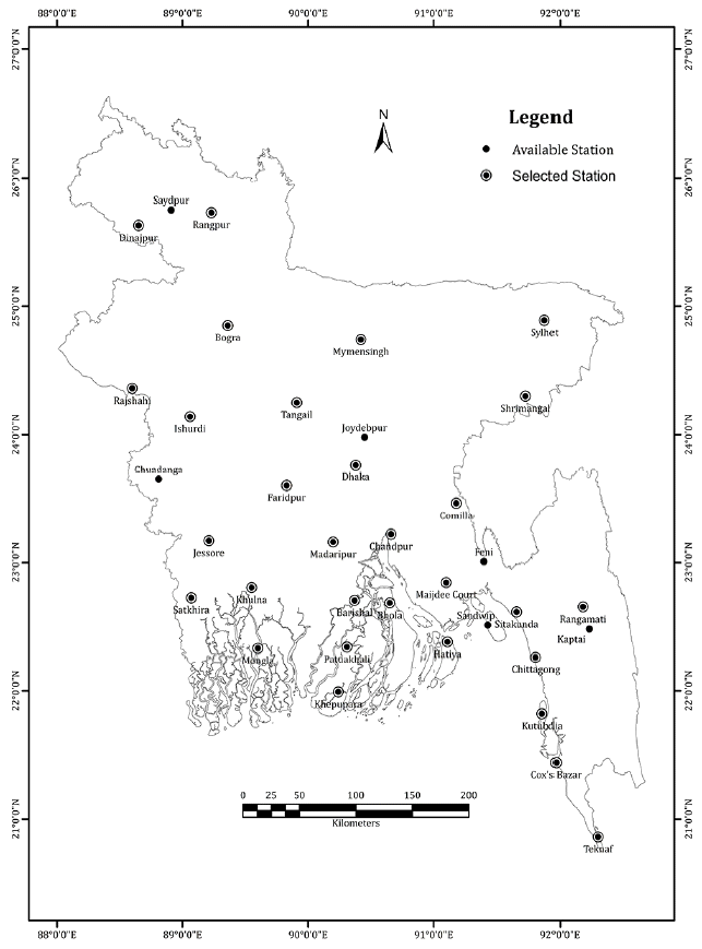
Quality control of data is an essential step before the calculation of indices because erroneous outliers can mislead the index calculation [11]. The key purpose of the quality control procedure was to identify errors in data processing, such as errors in manual keying [12]. As a first step, missing values were screened. Stations, containing more than 2% missing value were excluded from the modeling. Other checks such as identification of consecutive month with the same amount of rainfall along the year, the precipitation value below 0 mm, winter rainfall more than average rainfall and monsoon rainfall below the threshold limit were also carried out [10]. After checking these, thirty stations having long-term data (more than 20 y) up to the year 2013 and passing the above tests were used in the present study. Locations of the stations are shown in Fig. 1.
The homogeneity of the data series was identified using Standard Normal Homogeneity test [13], Von Neumann Ratio test [14], Buishand Range test [15] and Pettitt test [16]. The rainfall data sets of all the stations were found homogenous except for Shrimangal station. There was a breakpoint for Srimangal at 1961. Therefore, rainfall data from 1961 to 2013 was used for this station.
2.2. The ARIMA Model
Seasonal ARIMA model, proposed by Box and Jenkins [1] was used for model building and forecasting monthly rainfall. Seasonal ARIMA model can be labeled as ARIMA (p, d, q) * (P, D, Q)s where (p, d, q) is the nonseasonal part and (P, D, Q)s is the seasonal part of the model which could be written as:
Where, p = non-seasonal Auto Regressive (AR) order, d = non-seasonal differencing, q = non-seasonal Moving Average (MA) order, P = seasonal AR order, D = seasonal differencing, Q = seasonal MA order, and S = length of the season.
Building an ARIMA model consists of four systematic stages (identification, estimation, diagnostic check and application or forecast). The identification phase involves the improvement of the stationarity and normality of the data. At this stage, the general form of the model is estimated. Model parameters are calculated using the method of maximum likelihood at estimation stage. The diagnostic checks are performed to reveal the possible inadequacies and to select the best model. Finally, the forecasting of the rainfall time series is done.
3. Results and Discussion
3.1. Model Identification
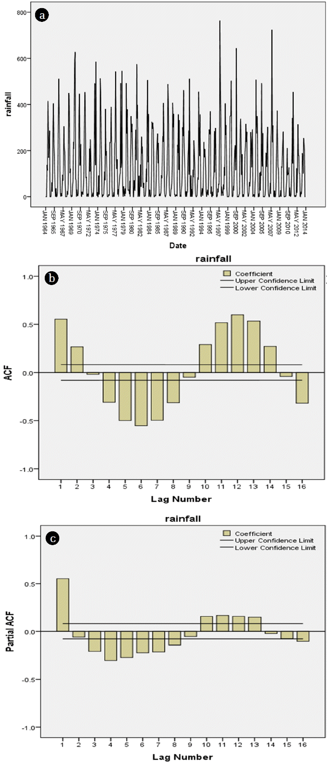
The identification stage involves checking the stationarity and normality of time series data. Initially, the data series were analyzed to check if the data are stationary and if there are any seasonality exists. The temporal correlation structure of the monthly time series was identified using Autocorrelation (ACF) and Partial Autocorrelation (PACF) Function [17]. Inspecting the time series plot, ACF, and PACF a clear seasonality of twelve months cycle was detected. Therefore, seasonal differencing of an appropriate order was done to remove seasonality and to achieve stationarity of data. A first order seasonal differencing was adequate to achieve stationarity for all the stations.
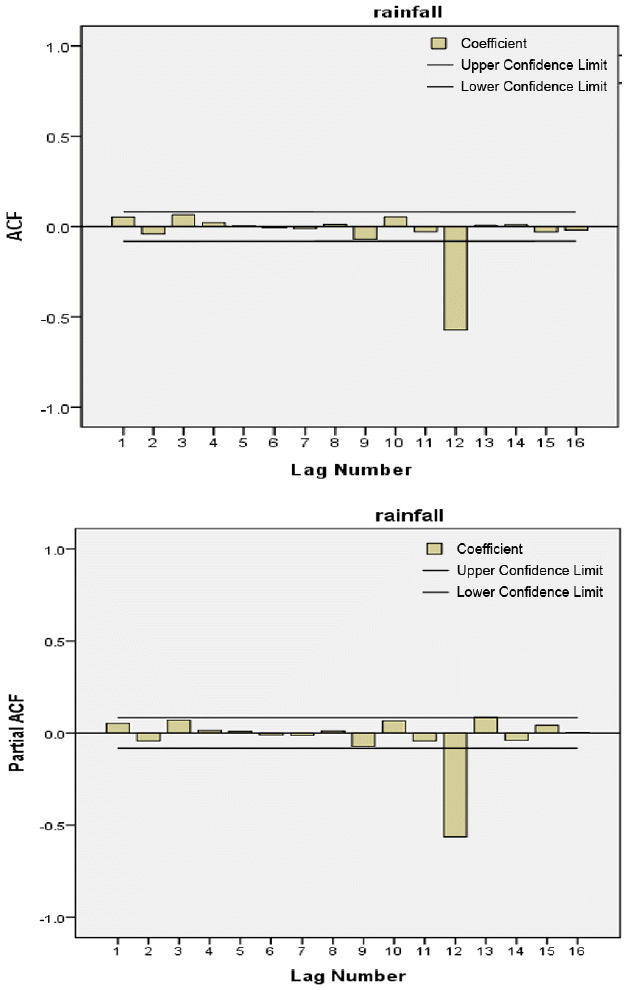
For example, time series plot of Rajshahi station is shown with ACF and PACF plots in Fig. 2. The sine-wave formation of ACF indicates that the data is seasonal. After a first order seasonal differencing ACF and PACF plot (Fig. 3) shows that the series is stationary. The ACF and PACF of the differenced series show no significant spikes indicating simplest Seasonal ARIMA process. However, the model could be a combination of both AR and MA process. The ACF and PACF plot direct a possible SARIMA model with P = 0–2 and Q = 0–2. All the possible combinations using several P and Q ranging from zero to two were examined to determine the best ARIMA model from the nominee models. The model that gives the best combination of minimum RMSE, maximum R-squared, and least Normalized BIC was selected as the best fit model.
3.2. Parameter Estimation
Primary estimation of the parameters was done from AR and MA at the identification stage. This preliminary evaluation was then used to compute the final parameter by the procedure described by Box and Jenkins (1976) [1]. The value of the parameters, standard error (SE), t-ratio, and p-values for each station are shown in Table 1. The standard error calculated for the relevant parameter is small compared to the parameter values. Therefore, the parameters are statistically significant [2].
3.3. Diagnostic Check
The diagnostic check was done once the model parameters were calculated to verify the adequacy of the prediction. The residuals should be white noise for a useful forecasting model. Several tests carried out on residuals are described below:
3.3.1. ACF and PACF of residuals
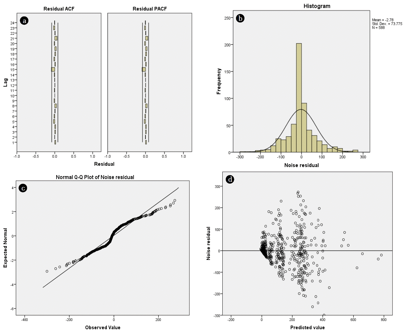
The majority of the ACF and PACF values of residuals lie within the confidence limit which indicates no significant correlation among them. Illustration of the ACF and PACF of residuals for rainfall series of Rajshahi station are given in Fig. 4. The figure shows that the residuals are white noise.
3.3.2. Histogram of residual
Histogram of residuals of rainfall series of Rajshahi station (Fig. 4(b)) shows that the residuals are normally distributed. Remaining series also exhibit similar result.
3.3.3. Normal probability of residuals
The cumulative distribution of the residuals data usually appears as a straight line when plotted on normal probability paper [18]. The normal probability plot of residuals were found fairly linear for all stations, indicating the residuals are normally distributed. Fig. 4(c) represents the normal probability of residuals for Rajshahi station.
3.3.4. Residuals versus prediction
Residuals were plotted against predicted values. The plot (Fig. 4(d)) for Rajshahi station shows that residuals are evenly distributed around mean, which indicate that the model is well fitted. Similar results were found for other stations also.
3.3.5. Lack of fit test
The modified Ljung Box statistics was used to verify the null hypothesis that the model is correctly specified [19]. The test statistics is shown in Table 2. The associated P-value is greater than 0.05 for maximum stations, which hold the null hypothesis of being white noise. The test indicates the models are adequate.
3.4. Rainfall Forecasting
The forecast is done for 12 months lead time, using the best model calculated from historical data. The plot between observed and predicted values (Rajshahi station) in Fig. 5 indicates that the predicted values follow the observed data closely enough. The performance criteria of the selected seasonal ARIMA model are shown in Table 2. The high value of R-square indicates the performance of the model is fair enough. The appropriateness of the models is confirmed by investigating Normalized BIC. The models have least BIC value, upheld the significance of the model. In addition to statistical terms, the performance of the developed models was compared with the available literature in the country (e.g. Bari et al. 2015 and Mahsin et al. 2012) and found sound in rainfall forecasting comparing to these.
4. Conclusions
Rainfall forecast becomes difficult in Bangladesh due to its non-linear pattern and the spatiotemporal variation in size. However, prediction of rainfall is necessary for flood management, rainwater harvesting, urban planning, water resource management, planning and optimal operation of the irrigation system. Considering the significance, rainfall forecasting using widely accepted ARIMA modeling technique is done in this paper. The highest R-squared value (0.868) was found for Teknaf station and the lowest value (0.672) was found for the Barishal station. Only two stations contain R-squared value below 0.70 which indicate the SARIMA models developed to forecast rainfall in the present study is reasonably precise. Hence, these SARIMA models can be used as a convenient tool for nationwide rainfall forecasting.


