Effects of hydrodynamics and coagulant doses on particle aggregation during a rapid mixing

Sang-Min Park; Tae-Young Heo; Jun-Gyu Park; Hang-Bae Jun

doi:10.4491/eer.2016.046

Environ Eng Res > Volume 21(4); 2016 > Article

Park, Heo, Park, and Jun: Effects of hydrodynamics and coagulant doses on particle aggregation during a rapid mixing

Research Article

Environmental Engineering Research 2016; 21(4): 365-372.

Published online: July 4, 2016

DOI: https://doi.org/10.4491/eer.2016.046

Effects of hydrodynamics and coagulant doses on particle aggregation during a rapid mixing

Sang-Min Park¹, Tae-Young Heo², Jun-Gyu Park³, Hang-Bae Jun^3,^†

¹Environmental Infrastructure Research Department, National Institute of Environmental Research(NIER), Incheon 22689, Republic of Korea

²Department of Information Statistics, Chungbuk National University, Cheongju 28644, Republic of Korea

³Department of Environmental Engineering, Chungbuk National University, Cheongju 28644, Republic of Korea

^†Corresponding author: Email: jhbcbe@cbnu.ac.kr, Tel: +82-43-261-2470 Fax: +82-43-261-2465

Received March 16, 2016 Accepted June 30, 2016

(open-access):

This is an Open Access article distributed under the terms of the Creative Commons Attribution Non-Commercial License (http://creativecommons.org/licenses/by-nc/3.0/) which permits unrestricted non-commercial use, distribution, and reproduction in any medium, provided the original work is properly cited.

Abstract

The effects of hydrodynamics and alum dose on particle growth were investigated by monitoring particle counts in a rapid mixing process. Experiments were performed to measure the particle growth and breakup under various conditions. The rapid mixing scheme consisted of the following operating parameters: Velocity gradient (G) (200–300 s⁻¹), alum dose (10–50 mg/L) and mixing time (30–180 s). The Poisson regression model was applied to assess the effects of the doses and velocity gradient with mixing time. The mechanism for the growth and breakup of particles was elucidated. An increase in alum dose was found to accelerate the particle count reduction. The particle count at a G value of 200 s⁻¹ decreased more rapidly than those at 300 s⁻¹. The growth and breakup of larger particles were more clearly observed at higher alum doses. Variations of particles due to aggregation and breakup of micro-flocs in rapid mixing step were interactively affected by G, mixing time and alum dose. Micro-flocculation played an important role in a rapid mixing process.

Keywords: Mixing time, Particle growth, Poisson regression, Rapid mixing scheme, Velocity gradient

1. Introduction

In conventional water treatment processes, rapid mixing is an important process that induces the instant dispersion of the coagulant and the destabilization of colloidal particles in water. It can also directly influence the removal of turbidity in the subsequent flocculation, sedimentation and filtration processes. The size of grown particles during rapid mixing influences the efficiency of membrane processes, especially. In case of Micro Filter (MF) process for water treatment, the complete blocking of particles is based on the premise that the particles size is larger than the pore size of the membrane [1]. Matsushita et al. [2] reported that long-duration mixing is probably not needed in the coagulation-MF hybrid system. That means, if the sizes of grown particles in a rapid mixing are suitable to optimum pore size of MF, operation of economical coagulation-MF hybrid process without long mixing time is possible. Rapid mixing involves both physical and chemical coagulation reactions. Because the hydrolysis of the coagulant, such as aluminium (III) or iron (III) salts, and the adsorption of hydroxide precipitates on colloidal particles occurs extremely quickly, rapid and uniform dispersion of the coagulant is essential for effective coagulation in a rapid mixing tank. Furthermore, the contact between the coagulant hydroxides and particles by physical collision, which induces particles growth, is also important.

Previous studies on mixing intensity and time have recommended a mixing time of less than 1 s and a velocity gradient (G) of 1,000 s⁻¹ based on the kinetics of the relevant electrochemical reactions, namely, the adsorption of hydroxides and charge neutralization of particles [3–5]. Amirtharajah and Mills [6] reported that particle destabilization could be achieved through the instant dispersion of the coagulant followed by the adsorption of aluminium hydroxides formed between 0.01 and 1.0 s after coagulant injection onto the surface of colloidal particles. They also suggested that instant dispersion and high agitation intensity were less important in sweep coagulation by hydroxide precipitate and that rapid mixing conditions were independent of coagulation efficiency. On the other hand, Camp [7] and Letterman et al. [8] suggested 1–2 min as a rapid mixing time to promote adequate floc characteristics for the subsequent flocculation and sedimentation processes. The American Society of Civil Engineers (ASCE) and the American Water Works Association (AWWA) recommended a velocity gradient of 700–1,000 s⁻¹ and mixing time of 20–60 s as a design guideline for rapid mixing tanks. Lai [9], however, noted that the mixing efficiencies for a given G and mixing time (t) were actually different. Mhaisalkar et al. [10] suggested an optimum combination of the G and mixing time for the practical treatment of turbid water. Furthermore, Rossini et al. [11] indicated that the duration of rapid mixing strongly influenced turbidity removal and determined the optimum combination of physical parameters. They confirmed that high turbidity removal could be achieved using both a short mixing time (approximately 10 s) and a long mixing time (approximately 60–90 s) using highly turbid synthetic water. Recently, Park et al. [12] investigated particle growth at different G values and mixing times using standard jar tests. At the predetermined optimum coagulant dose, they showed that the number of particles larger than 8.0 μm was lowest for a G value of 200 s⁻¹ and a mixing time of 150 s. The best turbidity removal was also confirmed under these rapid mixing conditions followed by flocculation and sedimentation processes. However, the number of these particles decreased for mixing times of over 180 s, most likely due to breakup, resulting in a deterioration of turbidity removal. Particles growth and breakup in a rapid mixing are influenced by several chemical and physical parameters, including coagulants dose, reactor geometry, mixer type, G and mixing time. Therefore, this study investigates the effects of hydrodynamics and coagulant dose on particle growth and examines their interrelation during rapid mixing.

2. Materials and Methods

2.1. Raw Water

A kaolin (Shinyo Chemical, Japan) suspension was used for the synthetic water samples. First, 5 g of kaolin was completely dispersed with vigorous agitation in 1 L of distilled water. The kaolin suspension was allowed to settle for 24 h, and 600 mL of the supernatant was sampled without disturbance. The decanted solution was diluted with tap water to adjust the sample turbidity to 10 NTU. The alkalinity was adjusted to 50 mg/L as CaCO₃ by adding NaHCO₃. The raw water samples were kept in suspension by gentle agitation at room temperature until use. Park et al. [12] reported that the particle size distribution of synthetic kaolin suspension was comparable to that of natural lake water samples. The characteristics of synthetic water and natural lake water are shown in Table 1.

2.2. Coagulants and Experimental Methods

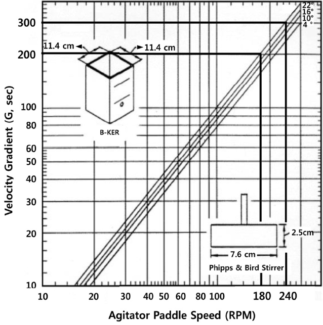
Coagulants based on aluminium are used in most water treatment plants in Republic of Korea. Therefore, the alum (Al₂(SO₄)₃·14H₂O), which is most typical coagulant based on aluminium, was used in this study. First, 1.0 % alum stock solution was prepared by dissolving Al₂(SO₄)₃·14H₂O in distilled water. The stock solution was diluted to 0.1 % alum solution before injection for each jar test. Several jar tests were conducted to investigate the behavior of particle growth at different coagulant doses and rapid mixing schemes. A square jar (L × W × H = 11.5 × 11.5 × 21 cm, Phipps & Bird) with a single-blade paddle (Fig. 1) and a variable-speed driving unit was used as a mixing device. The mixing intensity in terms of rotation velocity (RPM) was determined based on the G (G value) using the graphical method provided by Phipps & Bird Inc. (Fig. 1). The particle sizes and counts were investigated using a particle counter (PAMAS, Germany) at each rapid mixing step.

Rapid mixing was conducted at G values of 200 and 300 s⁻¹ for 180 s, corresponding to rotation velocities of 180 and 240 rpm, respectively. At different alum doses in the range of 10–50 mg/L, particle counts were analyzed every 30 s during the rapid mixing period. The growth of micro-floc was investigated by analyzing the particle size distribution in the range of 0.5 μm to 25.0 μm. Each rapid mixing experiment was conducted at pH 7.0 and room temperature (20 ± 1°C).

2.3. Poisson Regression

Poisson regression is a form of regression analysis used to model count data. Poisson regression assumes the response variable Y has a Poisson distribution. It hypothesizes that a sample of n observations, Y₁, Y₂, …, Y_n can be treated as realizations of independent Poisson random variables, with Y_i ~ Poisson(μ_i) and the mean μ_i depends on a set of k explanatory variables X_i. It is assumed that the logarithm of its expected value can be modelled by a linear combination of unknown parameters. The model takes the following form [13, 14]:

(1)

log (E (Y ∣ X)) = exp (β_{0} + β_{1} x_{1} + \dots β_{k} X_{k})

If Y is independent observations with a set of k corresponding values X of the exploratory variables, the unknown parameters β₀, β₁, ···, β_k can be estimated by maximum likelihood method. Wald chi-square values were used to test their significance in SAS PROC GENMOD.

3. Results and Discussion

3.1. Particle Counts during the Rapid Mixing

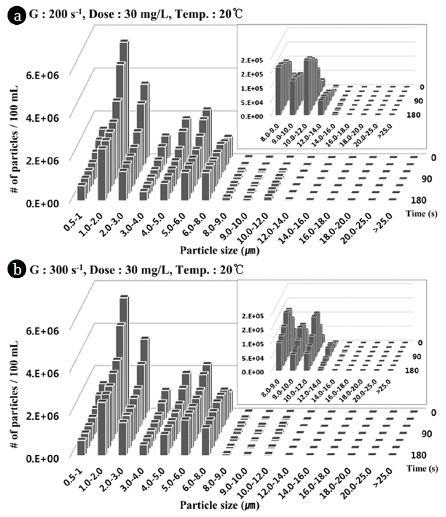
Fig. 2 shows typical trends for the particle counts during the rapid mixing as a function of mixing time at G values of a) 200 s⁻¹ and b) 300 s⁻¹ (pH, 7.0; dose, 30 mg/L; T, 20°C). The growth of micro-flocs was clearly observed at both G values, as the total particle counts decreased with rapid mixing time. The particle counts of the smaller particles (i.e., 0.5–6.0 μm) decreased with rapid mixing time, indicating that aggregation (micro-flocculation) of micro-flocs could occur by interparticle collision despite the very intense mixing. Micro-flocculation (also known as perikinetic flocculation), in which particle aggregation occurs due to the random thermal motion of fluid molecules, can be identified by the particles smaller than micro-eddy size, η (= (ν/G)^1/2), in the mixing tank. In this study, the η values at 20°C were approximately 71 and 58 μm, corresponding to G values of 200 and 300 s⁻¹, respectively. Therefore, the particle aggregation could be classified as micro-flocculation. These observations suggest that hydrodynamics and mixing time play an important role in the collisions between instantaneously formed alum hydroxide precipitates and colloidal kaolin particles, which is then followed by the growth of micro-flocs during the rapid mixing step.

There was no significant change in the counts of particle sizes 6.0–8.0 μm during the overall period of jar-test at G values of 200 and 300 s⁻¹, respectively. Thus, particle sizes 6.0–8.0 μm would be considered about turning point from breakup to growth of particles. In case of the counts of particles smaller than 6.0 μm were decreased during the overall period of jar-test at G values of 200 and 300 s⁻¹. Thus, a sufficiently long mixing time provides the collisions of particles smaller than 6.0 μm necessary for the growth of flocs by aggregation. On the other hand, the counts of particles larger than 8.0 μm at G values of 200 and 300 s⁻¹ started to increase after 30 s and 0 s, respectively. The counts of medium-sized particles (8.0–16.0 μm) steadily increased with mixing time at a G value of 200 s⁻¹ but began to decrease after 90 s at a G value of 300 s⁻¹. The growth behavior of these particles was slightly different for different G values. Based on the counts of particles larger than 18.0 μm, the grown flocs might break up after 90–120 s. The breakup of these particles may adversely affect the aggregation and growth of flocs in the rapid mixing step. The operating parameters in rapid mixing, such as alum dose, mixing intensity and mixing time, are interactive. Thus, they may affect the efficiency of the flocculation and sedimentation of macro-flocs in the subsequent processes. Indeed, an increase in larger particles over 8.0 μm indicated better turbidity removal in a previous study [10]. It is necessary to optimize the operating parameters to grow larger flocs without breakup.

3.2. Poisson Regression Model with Particle Counts

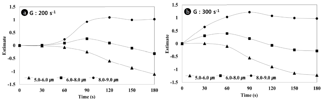
This study demonstrates the use of a Poisson regression model to evaluate the effect of hydrodynamics and alum dose on particle counts. A Poisson regression model was used to identify the dose and G conditions affecting particle growth and breakup during the rapid mixing period. The parameter estimates of mixing time in the Poisson regression model were obtained for doses from 10 to 50 mg/L as a function of rapid mixing at two Gs (G values of 200 and 300 s⁻¹). The sign of the parameter estimates over mixing time in the model changed as the particle counts varied relative to the particle counts at mixing time 0 (particle counts in raw water). Positive estimates denote a positive effect on particle counts, meaning that the particle counts are greater than those at mixing time 0, whereas negative estimates have the opposite meaning. Fig. 3 –5 show that the effect of mixing time on particles counts of near a turning point (6.0–8.0 μm) at two Gs for alum doses of 10, 30 and 50 m/L, respectively. In addition, Tables 2 –4 show particle counts of the rest of size distributions. Therefore, the sign of the parameter estimates in the Poisson regression model indicates the effect of mixing time on particle count by dose and G. In Fig. 3, particle counts of sizes 5.0–6.0 μm at all of two G values decreased with mixing time. Additionally, the particle counts decreased more quickly at a G value of 300 s⁻¹ than at a G value of 200 s⁻¹. The particle counts gradually decreased until 30–60 s and then rapidly decreased after 90 s. A turning point exists at sizes 6.0–8.0 μm, where the sign of the parameter estimates changes from negative to positive. Specifically, the turning times were 90 s and 60 s at G values of 200 s⁻¹ and of 300 s⁻¹, respectively. Based on the negative estimate at each mixing time, the particle counts of sizes 8.0–9.0 μm increased with mixing time relative to that at time 0. The particle counts of sizes 8.0–9.0 μm increased more rapidly at a G value of 300 s⁻¹ than at a G value of 200 s⁻¹. When the particle size was relatively large, patterns of particle growth and breakup were clearly observed.

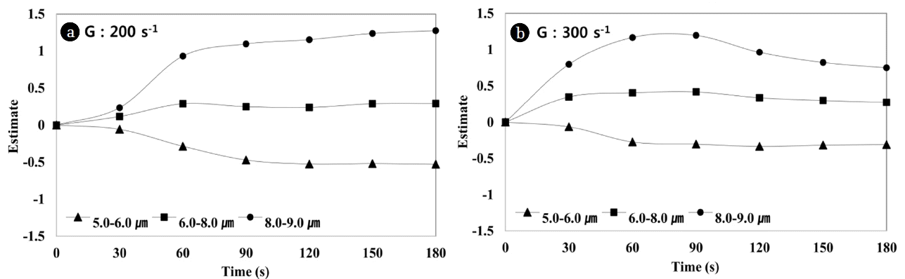
The Poisson regression model was also used to obtain parameter estimates as a function of mixing time for a dose of 30 mg/L (Fig. 4 and Table 3). The particle counts decreased with mixing time for particles smaller than size of 6.0 μm, similarly to those at a dose of 10 mg/L. Unlike dose 10 mg/L, however, at dose 30 mg/L, there is no difference in the decreasing pattern of the particle counts for particle sizes of 0.5–2.0 μm or a G value of 200 s⁻¹ and a G value of 300 s⁻¹ (Table 3). The counts of particles larger than size of 2.0 μm decrease more rapidly at a G value of 200 s⁻¹ than those at a G value 300 s⁻¹, which was contrary to the pattern at dose 10 mg/L. The turning point for the increase in particle count was observed at size of 6.0–8.0 μm for G values of 200 s⁻¹ and 300 s⁻¹, which was comparable to the trend for dose 10 mg/L. At a G value of 200 s⁻¹, the counts of medium-sized particles (8.0–16.0 μm) increased with mixing time. In contrast, at a G value of 300 s⁻¹, the particle counts increased until 120 s and then decreased.

For particle sizes of 0.5–1.0 μm, an increase and decrease in particle count, similar to those at dose 10 mg/L, were observed at G values of 200 s⁻¹ and 300 s⁻¹ due to the growth and breakup of larger particles. Because the created particle counts at dose 10 mg/L are relatively small, the particle counts for sizes of 0.5–4.0 μm decreased more rapidly at a G value of 300 s⁻¹. The particle counts for particle sizes of 0.5–2.0 μm decreased at the same rate at G values of 200 s⁻¹ and 300 s⁻¹, whereas the particle counts at a G value of 300 s⁻¹ decreased more rapidly for particle sizes of 2.0–6.0 μm than those at a G value of 200 s⁻¹. The reason for this difference is that larger particles break more easily, increasing the small-particle counts at a G value of 300 s⁻¹. Although the particle count gradually and continuously increased for a G value of 300 s⁻¹, a turning point exists for particle sizes of 8–13 for a G value of 200 s⁻¹. This pattern shows that medium-sized particles (8.0–16.0 μm) at a G value of 300 s⁻¹ began to break up at extended mixing times, which increased the particle counts in the range of 2.0–6.0 μm relative to those at 200 s⁻¹. Furthermore, the particle counts at dose 10 mg/L changed more rapidly than those at dose 30 mg/L. Accordingly, the alum dose affected particle growth and breakup in the rapid mixing period.

As shown in Fig. 5 and Table 4, the particle counts continuously decreased until particle size of 5.0 μm at a dose of 50 mg/L, similarly to the results for the other doses. However, the decreasing pattern was different from that at dose 10 mg/L for G values of 200 s⁻¹ and 300 s⁻¹. At dose 50 mg/L, the particle counts at a G value of 200 s⁻¹ decreased more rapidly than those at 300 s⁻¹. Furthermore, a turning point from breakup to aggregation at dose 50 mg/L was formed at smaller particle size (5.0–6.0 μm) than dose 10 mg/L and 30 mg/L. The higher dose of coagulant causes the charge reversal in water [15]. Moreover, the charge reversal leads the thin double layer and breakup of particles [16]. Ranran Mao et al. reported that the higher coagulant dosage would be lead the small floc size and loose structure. They confirmed that floc size was decreased about 1/3 at higher coagulant dosage comparison with optimum dosage [17].

The particle counts increased for particle sizes of 8.0–20.0 μm at a G value of 200 s⁻¹. However, the sign of the change from positive to negative was observed at a mixing time of 120 s for particle sizes of 6.0–8.0 μm. Moreover, there was another sign change from negative to positive for particle sizes of 14.0–16.0 μm at a G value of 300 s⁻¹. Therefore, particle growth and breakup were significant at a dose of 50 mg/L. The decrease in particle count at this dose was slower than that at the lower doses of 10 mg/L and 30 mg/L, interestingly.

Micro-flocculation occurred in a rapid mixing step with different patterns for various combinations of G (G value), mixing time (t) and alum dose. Several researchers [3, 4] suggested very short mixing times (less than 1 s) for the rapid mixing of metallic coagulants based on their quick chemical reactions in water. Several operating and design guidelines (ASCE, AWWA) for rapid mixing recommended G values of 700–1,000 s⁻¹ and mixing times of less than 60 s. These suggestions are based on the uniform distribution of the coagulant before its chemical reactions in the water. A high G and short rapid mixing time for alum coagulation appears to be very reasonable based on its chemical reactions; however, micro-flocculation during rapid mixing would also play an important role in the subsequent flocculation and sedimentation processes. The G, mixing time and alum dose affect micro-flocculation during rapid mixing. For optimum micro-flocculation, a relatively low alum dose (less than 30 mg/L) and G value (less than 300 s⁻¹) for a prolonged rapid mixing time (120–150 s) were found most effective in this study.

For the sweep floc coagulation normally used in field, alum overdose is usually applied to rapidly form precipitates and enhance flocculation efficiency. Especially for enhanced coagulation intended to reduce disinfection by-products, a high G and extended mixing time, as shown in the literature, might induce micro-floc breakup in rapid mixing. Particles of 1.0 and 2.0 μm in size in raw water collide innumerable times with other particles and grow into settleable flocs (several mm in size). The destabilization of the charged particles in raw water is a prerequisite of these collisions, and a higher dose of alum and rapid mixing are required for the rapid growth of micro-flocs. The breakup of the micro-flocs starts from the rapid mixing steps at higher alum doses, higher G values and/or extended mixing times.

4. Conclusions

The effects of hydrodynamics and alum dose on the changes in particle counts with time were investigated in a rapid mixing period. A decrease in particle counts due to the collision and aggregation of smaller micro-flocs was clearly observed despite the high mixing intensity, followed by an increase in larger particle counts. In addition to the G value and alum dose, the mixing time strongly affected both micro-floc growth and breakup, especially at extended mixing times. The interrelations among the variations for rapid mixing were sufficiently complicated that a Poisson regression model was applied to analyze the particle growth and breakup. The conclusions are as follows:

Higher alum doses resulted in higher total particle counts during the rapid mixing period.
At the same alum dose, the growth rate of micro-flocs at a G value of 300 s⁻¹ was higher than that at a G value of 200 s⁻¹ based on the total particle counts. However, breakup of the grown flocs at a G value of 300 s⁻¹ occurred earlier than that at 200 s⁻¹.
Particles smaller than 6.0–8.0 μm gradually decreased at earlier mixing times and rapidly decreased at later mixing times at a dose of 10 mg/L. However, the particle counts at doses of 30 mg/L and 50 mg/L rapidly decreased. As the alum dose increased, the particle count reduced rapidly slowed.
The decrease in particle counts for a G value of 200 s⁻¹ was more rapid than that for 300 s⁻¹.
The growth and breakup of large flocs were more active at relatively low dose of 10 mg/L.

Acknowledgements

Statistical analysis and interpretation were completed with the assistance of the Statistical Analysis and Consulting Center in Chungbuk National University.

References

1. Sampath M, Shukla A, Rathore AS. Modeling of filtration processes–Microfiltration and depth filtration for harvest of a therapeutic protein expressed in pichia pastoris at constant pressure. Bioengineering. 2014;1:260–277.

2. Matsushita T, Matsui Y, Shirasaki N, Kato Y. Effect of membrane pore size, coagulation time, and coagulant dose on virus removal by a coagulation-ceramic microfiltration hybrid system. Desalination. 2005;178:21–26.

3. Hudson H, Wolfner JP. Design of mixing tank and flocculation basins. J Am Water Works Assoc. 1976;59:1257.

4. Vrale L, Jarden RM. Rapid mixing in water treatment. J Am Water Works Assoc. 1971;63:52–58.

5. Kawamura S. Consideration in improving flocculation. J Am Water Works Assoc. 1976;68:328–336.

6. Amirtharajah A, Mills KM. Rapid mix design for mechanisms of alum coagulation. J Am Water Works Assoc. 1982;74:210–216.

7. Camp TR. Floc volume concentration. J Am Water Works Assoc. 1968;60:656–673.

8. Letterman RD, Quon JK, Gemmel RC. Influence of rapid mix parameters on flocculation. J Am Water Works Assoc. 1973;65:716–725.

9. Lai RJ, Hudson HE, Singley JE. Velocity gradient calibration of jar-test equipment. J Am Water Works Assoc. 1975;67:553–557.

10. Mhaisalkar VA, Paramasivam R, Bhloe AG. Optimizing physical parameters of rapid mix design for coagulation-flocculation of turbid waters. Water Res. 1991;25:43–52.

11. Rossini M, Garcia Garrido J, Galluzzo M. Optimization of the coagulation-flocculation treatment: Influence of rapid mix parameters. Water Res. 1999;33:1817–1826.

12. Park SM, Jun HB, Jung MS, Koo HM. Effects of velocity gradient and mixing time on particle growth in a rapid mixing tank. Water Sci Technol. 2006;53:95–102.

13. McCullagh P, Nelder JA. Generalized linear models. 2nd edNew York: Chapman and Hall; 1989.

14. Liley JB. Fitting size distributions to optical particle counter data. Aerosol Sci Technol. 1992;17:84–92.

15. Christian S, Mathias H, Bastian W, Arben J, Matthias B. Experimental study of electrostatically colloidal particles: Colloidal stability and charge reversal. J Colloid Interf Sci. 2011;358:62–67.

16. Lopez-Garcia JJ, Arandra-Rascon MJ, Grosse C, Horno J. Electrokinetics of charged colloidal particles taking into account the effect on ion size constraints. J Colloid Interf Sci. 2011;356:325–330.

17. Ranran M, Yan W, Bo Z, Weiying X, Min D, Baoyu G. Impact of enhanced coagulation ways on flocs properties and membrane fouling: Increasing dosage and applying new composite coagulant. Desalination. 2013;314:161–168.

Fig. 1

Square jar (2 L) for batch tests (Phipps & Bird) and velocity gradient in terms of RPM (Phipps & Bird).

Fig. 2

Particle size distribution at G values of a) 200 s⁻¹ and b) 300 s⁻¹.

Fig. 3

Effects of particle aggregation at turning point (size 6.0–8.0 μm) on time and G [a) 200 s⁻¹, b) 300 s⁻¹] at dose 10 mg/L. Size: 5.0–6.0 μm; 6.0–8.0 μm; 8.0–9.0 μm. The Y-axis represents the parameter estimates of mixing time in the Poisson regression model. The estimate of mixing time 0 is always 0, corresponding to the baseline (horizontal dotted line). Standard errors of all results are ± 0.004.

Fig. 4

Effects of particle aggregation at turning point (size 6.0–8.0 μm) on time and G [a) 200 s⁻¹, b) 300 s⁻¹] at dose 30 mg/L. Size: 5.0–6.0 μm; 6.0–8.0 μm; 8.0–9.0 μm. The Y-axis represents the parameter estimates of mixing time in the Poisson regression model. The estimate of mixing time 0 is always 0, corresponding to the baseline (horizontal dotted line). Standard errors of all results are ± 0.004.

Fig. 5

Effects of particle aggregation at turning point (size 6.0–8.0 μm) on time and G [a) 200 s⁻¹, b) 300 s⁻¹] at dose 50 mg/L. Size: 5.0–6.0 μm; 6.0–8.0 μm; 8.0–9.0 μm. The Y-axis represents the parameter estimates of mixing time in the Poisson regression model. The estimate of mixing time 0 is always 0, corresponding to the baseline (horizontal dotted line). Standard errors of all results are ± 0.004.

Table 1

Characteristics of Raw Water

Item	Synthetic raw water	Natural lake water
Turbidity (NTU)	10	10
pH	7.75	8.14
Temperature (°C)	20	22.2
Alkalinity (mg/L as CaCO₃)	50–55	45–50

Table 2

Effects of Time and G for Various Sizes at Dose 10 mg/L

Particle Size(μm)	Time, sec (G = 200 s⁻¹)

	0	30	60	90	12	150	180
0.5–1.0	-	0.0003	−0.1035	−0.2049	−0.3626	−0.5784	−0.8085
1.0–2.0	-	−0.0194	−0.099	−0.3187	−0.5899	−0.8619	−1.1092
2.0–3.0	-	−0.0315	−0.1534	−0.4464	−0.8015	−1.105	−1.3531
3.0–4.0	-	−0.035	−0.1584	−0.4568	−0.8258	−1.1243	−1.3656
4.0–5.0	-	−0.0294	−0.1426	−0.4167	−0.7894	−1.0878	−1.3243
5.0–6.0	-	−0.0135	−0.0724	−0.2483	−0.5917	−0.8656	−1.1046
6.0–8.0	-	0.0081	0.0914	0.2605	0.0926	−0.1051	−0.3086
8.0–9.0	-	0.0066	0.2337	0.9215	1.0826	0.9883	1.0162
9.0–10.0	-	0.0213	0.2878	1.145	1.4323	1.4123	1.4844
10.0–12.0	-	−0.0038	0.2914	1.4443	2.0154	2.1115	2.0698
12.0–14.0	-	0.1196	0.231	1.8499	2.0339	3.4149	3.5112
14.0–16.0	-	0.497	0.3443	2.1065	4.0701	4.8063	5.0999
16.0–18.0	-	0	0.47	1.1838	3.9741	5.1743	5.6391
18.0–20.0	-	1.9454	2.5649	2.3026	5.0239	6.5653	7.2385
20.0–25.0	-	1.3863	0.6931	0.9163	3.0445	4.7493	5.8126
> 25.0	-	−0.2877	−23.6889	−1.3863	0.6931	1.3218	1.9095

Particle Size(μm)	Time, sec (G = 300 s⁻¹)

	0	30	60	90	12	150	180
0.5–1.0	-	−0.0739	−0.1222	−0.4211	−0.6396	−1.017	−1.1651
1.0–2.0	-	−0.0732	−0.1834	−0.6251	−0.9415	−1.1332	−1.4881
2.0–3.0	-	−0.1453	−0.3046	−0.8181	−1.161	−1.5034	−1.6362
3.0–4.0	-	−0.1309	−0.3026	−0.8215	−1.1802	−1.4929	−1.6172
4.0–5.0	-	−0.1019	−0.2581	−0.7734	−1.1392	−1.4264	−1.5292
5.0–6.0	-	0.0048	−0.1019	−0.5513	−0.8916	−1.1475	−1.2262
6.0–8.0	-	0.3013	0.3929	0.1934	−0.0685	−0.2432	−0.2846
8.0–9.0	-	0.6397	1.0266	1.2151	1.0715	0.9877	0.969
9.0–10.0	-	0.7464	1.2347	1.5848	1.4958	1.4448	1.4407
10.0–12.0	-	0.8606	1.5089	2.1598	2.1755	2.1859	2.1936
12.0–14.0	-	1.0533	1.9095	3.1599	3.3461	3.4713	3.4749
14.0–16.0	-	1.369	2.2916	4.1892	4.5737	4.8116	4.7735
16.0–18.0	-	1.3863	1.596	4.1368	4.6784	4.99	4.9205
18.0–20.0	-	2.9957	3.4657	5.2417	5.7683	6.2934	6.0707
20.0–25.0	-	2.0149	1.6094	3.4012	3.7377	4.3883	4.151
> 25.0	-	0	−0.6931	0	0.6931	0	1.0116

Table 3

Effects of Time and G for Various Sizes at Dose 30 mg/L

Particle Size(μm)	Time, sec (G = 200 s⁻¹)

	0	30	60	90	120	150	180
0.5–1.0	-	−0.1339	−0.3571	−0.5376	−0.5887	−0.6326	−0.6583
1.0–2.0	-	−0.1406	−0.4828	−0.6995	−0.7519	−0.7733	−0.7954
2.0–3.0	-	−0.1832	−0.592	−0.8254	−0.8805	−0.9009	−0.9202
3.0–4.0	-	−0.1735	−0.5789	−0.8058	−0.8622	−0.8756	−0.8908
4.0–5.0	-	−0.1445	−0.5119	−0.7391	−0.798	−0.8019	−0.8164
5.0–6.0	-	−0.0574	−0.2857	−0.4716	−0.5259	−0.5199	−0.5292
6.0–8.0	-	0.1159	0.2887	0.249	0.2385	0.2885	0.2923
8.0–9.0	-	0.2352	0.9313	1.0959	1.154	1.2372	1.2755
9.0–10.0	-	0.2625	1.1216	1.358	1.4527	1.5459	1.5789
10.0–12.0	-	0.2678	1.3058	1.6862	1.8266	1.9422	1.9862
12.0–14.0	-	0.2355	1.5036	2.0999	2.3166	2.4571	2.4928
14.0–16.0	-	0.3247	1.6176	2.2971	2.6143	2.7386	2.8178
16.0–18.0	-	0.2877	0.8473	1.4351	2.0711	2.0015	2.2119
18.0–20.0	-	2.1972	1.7918	2.5649	3.2189	2.9957	2.8332
20.0–25.0	-	0.4055	0.6931	1.5041	1.5041	1.5041	1.6094
>25.0	-	−0.6931	−0.6931	−0.6731	0.2231	0.5596	−0.6931

Particle Size(μm)	Time, sec (G = 300 s⁻¹)

	0	30	60	90	12	150	180
0.5–1.0	-	−0.1512	−0.4505	−0.5532	−0.6226	−0.6431	−0.6593
1.0–2.0	-	−0.1979	−0.5463	−0.6386	−0.7376	−0.7589	−0.774
2.0–3.0	-	−0.284	−0.6454	−0.7205	−0.7967	−0.8036	−0.8039
3.0–4.0	-	−0.2651	−0.6105	−0.6704	−0.7456	−0.7392	−0.7362
4.0–5.0	-	−0.2219	−0.5316	−0.5879	−0.6435	−0.63	−0.6238
5.0–6.0	-	−0.0651	−0.2744	−0.3041	−0.3349	−0.3178	−0.3099
6.0–8.0	-	0.3475	0.404	0.4162	0.3355	0.2976	0.2711
8.0–9.0	-	0.7964	1.1668	1.1954	0.9622	0.8226	0.7488
9.0–10.0	-	0.9275	1.3804	1.4307	1.1172	0.9403	0.8426
10.0–12.0	-	1.0801	1.6517	1.6752	1.2229	0.9959	0.8451
12.0–14.0	-	1.3008	1.9592	1.9966	1.1976	0.8791	0.6727
14.0–16.0	-	1.711	2.2433	2.2123	1.0519	0.74	0.7
16.0–18.0	-	1.7918	1.7346	2.0794	0.47	0.6592	0.4274
18.0–20.0	-	2.9957	3.3322	3.4012	2.6391	2.7081	2.5649
20.0-25.0	-	2.3514	2.3026	2.2513	1.6094	1.7918	1.3863
> 25.0	-	0.6931	0.6931	0.2231	−1.3863	0	0.4055

Table 4

Effects of Time and G for Various Sizes at Dose 50 mg/L

Particle Size(μm)	Time, sec (G = 200 s⁻¹)

	0	30	60	90	120	150	180
0.5–1.0	-	−0.1279	−0.2855	−0.3301	−0.3616	−0.355	−0.3476
1.0–2.0	-	−0.1255	−0.3351	−0.3921	−0.4299	−0.4151	−0.4045
2.0–3.0	-	−0.1584	−0.385	−0.4456	−0.492	−0.4767	−0.4722
3.0–4.0	-	−0.1458	−0.3542	−0.4166	−0.4576	−0.4364	−0.4293
4.0–5.0	-	−0.1246	−0.2931	−0.3443	−0.3831	−0.3622	−0.3606
5.0–6.0	-	−0.0588	−0.1169	−0.1411	−0.1504	−0.122	−0.1217
6.0–8.0	-	0.0337	0.2322	0.2732	0.3406	0.4027	0.4101
8.0–9.0	-	0.0552	0.5085	0.6117	0.7937	0.8818	0.9122
9.0–10.0	-	0.0676	0.5655	0.695	0.8882	0.9939	1.0293
10.0–12.0	-	0.066	0.552	0.6633	0.9474	1.0919	1.126
12.0–14.0	-	0.0572	0.5359	0.5763	0.9781	1.0858	1.1634
14.0–16.0	-	0.4191	0.8155	0.6148	1.1985	1.3117	1.4903
16.0–18.0	-	0.1823	0.9295	0.6592	0.9295	1.0761	1.2432
18.0–20.0	-	1.3863	1.6094	1.7918	2.4849	2.3979	2.9957
20.0–25.0	-	−0.6931	0	0.4055	1.3863	1.3863	0.9163
> 25.0	-	−25.6889	0	−1.3863	−1.3863	−1.3863	0

Particle Size(μm)	Time, sec (G = 300 s⁻¹)

	0	30	60	90	12	150	180
0.5–1.0	-	−0.1507	−0.2462	−0.2542	−0.2604	−0.2891	−0.2973
1.0–2.0	-	−0.1683	−0.2582	−0.2694	−0.2737	−0.306	−0.3167
2.0–3.0	-	−0.2326	−0.3021	−0.301	−0.2802	−0.3024	−0.3168
3.0–4.0	-	−0.2034	−0.2661	−0.2622	−0.2502	−0.2679	−0.2761
4.0–5.0	-	−0.1635	−0.2003	−0.2002	−0.2024	−0.2159	−0.2309
5.0–6.0	-	−0.022	−0.0224	−0.0253	−0.1053	−0.123	−0.143
6.0–8.0	-	0.3026	0.3775	0.336	−0.0474	−0.0859	−0.1241
8.0–9.0	-	0.6445	0.764	0.667	−0.16	−0.2333	−0.2953
9.0–10.0	-	0.727	0.8634	0.7811	−0.2245	−0.27	−0.3741
10.0–12.0	-	0.8416	0.9922	0.8844	−0.3862	−0.4144	−0.4473
12.0–14.0	-	1.033	1.1663	1.0489	−0.4649	−0.5493	−0.4835
14.0–16.0	-	1.4621	1.6628	1.5296	−0.0278	−0.0278	0.0136
16.0–18.0	-	1.6227	1.6614	1.5404	0.383	0.0645	0.4274
18.0–20.0	-	3.0445	3.1355	3.091	2.3979	1.7918	1.6094
20.0–25.0	-	2.3016	1.8718	2.1401	1.2528	0.4055	0.9163
> 25.0	-	0	0	0.4055	−0.6931	0.2231	0.5596